Monte Carlo Simulation with Risk Kit

1. The Need to Be Able to Easily Create Monte Carlo Simulations

Monte Carlo simulations play an increasingly important role in finance, the social sciences, and risk management. Monte Carlo simulation is a generic method for estimating the probability distributions of arbitrary target quantities in complex environments; these include, for example, profit distributions, firm value distributions, portfolio loss distributions, and, in general, the distribution of any target quantity subject to randomness.

Using Monte Carlo simulations in practice, however, is often subject to serious difficulties, such as the need to generate random numbers, program a model, and evaluate the simulation results. Solving these problems requires handling mathematical methods as well as modern computer technology.

Risk Kit is a tool for quickly and easily creating risk analyses and Monte Carlo simulations. It provides the components required for quantitative risk management and lets you combine them, in a simple and intuitive way, into complete models and risk analyses. Risk Kit gives many users efficient access to quantitative risk management and Monte Carlo simulations. It speeds up development time many times over compared with conventional approaches.

All Risk Kit functions can be integrated into the spreadsheet as cell functions in Microsoft Excel. In addition, Risk Kit functions can be called from VBA or embedded as a .NET assembly in production environments.

This article uses an example to describe how Monte Carlo simulations and risk analyses can be carried out with Risk Kit1.

2. Introducing Risk Kit

Risk Kit is an add-in for Microsoft Excel. Once installed, it is available in Excel via the Risk Kit ribbon.

Figure 1: The Risk Kit ribbon in Microsoft Excel.

In addition, the cell context menu contains a 'Risk Kit' submenu that also includes the ribbon's functions:

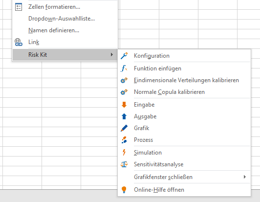
Figure 2: Cell context menu.

The following table describes all the buttons on the Risk Kit ribbon:

Button	Description
	Opens the function dialog box for selecting Risk Kit cell functions.
	Opens the gallery of one-dimensional distributions, where you can select a distribution to draw random variables or calculate the density, mass function, cumulative distribution function, or inverse cumulative distribution function.
	Opens the list of functions for stochastic processes.
	Opens the list of statistical functions.
	Opens the list of general functions, for example, for creating plots.
	Opens additional functions, grouped by multivariate distributions, rating procedures, and interest rate calculations.
	Opens the most recently used functions.
	Opens the calibration dialog box, which lets you calibrate univariate and multivariate distributions to empirical data.
	Marks a cell as an input cell.
	Marks a cell as an output cell.
	Marks a cell as a chart cell
	Marks a cell as a process cell
	Opens the cell manager to display Risk Kit function cells in the open workbooks.
	Opens the configuration dialog box, which lets you set simulation parameters, change the user interface language, and more.
	Starts the simulation.
	Performs a single step in the simulation.
	Resumes the simulation. The button is enabled when the simulation is paused.
	Cancels the simulation. The button is enabled when the simulation is paused.
	Opens the sensitivity analysis dialog box.
	The button provides a dropdown list with six items: 'Arrange Chart Windows' arranges the windows so that all charts are visible at once; 'Cascade Chart Windows' cascades the chart windows behind one another; 'Close Chart Windows' closes all chart windows; 'Delete Charts from the Active Worksheet' deletes the embedded charts from the active worksheet; 'Delete Charts from the Active Workbook' deletes the embedded charts from the active workbook; 'Delete Charts from All Open Workbooks' deletes the embedded charts from all open workbooks.
	Contains a variety of example workbooks to help you get started quickly with Risk Kit.
	Opens Risk Kit's add-in tools, where you can open the online help, change the interface language among English, French, and German, create keyboard shortcuts, send feedback to Risk Kit's developers, recommend Risk Kit to new users, troubleshoot problems, and view information about the Risk Kit version in use.

To run a Monte Carlo simulation of a previously deterministic model with Risk Kit, we proceed in four steps. First, you need to identify one or more inputs of the model that become random variables in the simulation. Their previous deterministic value is replaced in the simulation by random numbers that change with every simulation run. These variables are what introduce uncertainty into the model.

Second, you need to define the model results, or target quantities. They are calculated from the random inputs and, where applicable, other input quantities in the context of the model.

Third, you need to choose a number of simulation runs, so that, fourth, the simulation can be started.

3. A Profit and Loss Simulation

3.1. A Deterministic Model as a Starting Point

To give an example of how a deterministic model is extended into a Monte Carlo simulation, let's look at a simple profit and loss statement.

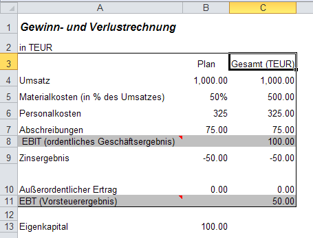
Figure 3: Deterministic profit and loss statement.

To calculate the company's profit and loss, we start with the company's revenue (C4) and deduct all costs from it. As a first step, these are material costs (C5) and personnel costs (C6), as well as depreciation (C7), which lead to the ordinary operating result before interest and taxes ('earnings before interest and taxes' (EBIT)) (C8). Finally, the interest result (C9) is deducted from this, and extraordinary income (C10) is added, to arrive at the pretax profit ('earnings before taxes' (EBT)) (C11). All formulas are simple sums and differences.

Since actual material costs are largely variable and depend on the level of revenue, we model them as a relative quantity, 'as a % of revenue'. The absolute material costs are then C5 = B5 * C4.

3.2. The Sources of Uncertainty

Once the deterministic model is defined, the first step toward a Monte Carlo simulation is to identify the sources of uncertainty in the model.

We assume that revenue, material costs, personnel costs, and extraordinary income are subject to uncertainty (column B). The goal is to determine their effect on the ordinary operating result and the overall result before taxes (column C). Note that risks can also occur as opportunities (for example, random cost relief) that increase profit.

While the deterministic model assumed a profit of 1,000 TEUR, we know from experience that this quantity is not constant but fluctuates randomly in practice, for example, between 900 and 1,050 TEUR, with 1,000 TEUR being the 'most likely value'. We therefore choose a triangular distribution as an intuitive model for the revenue fluctuations.

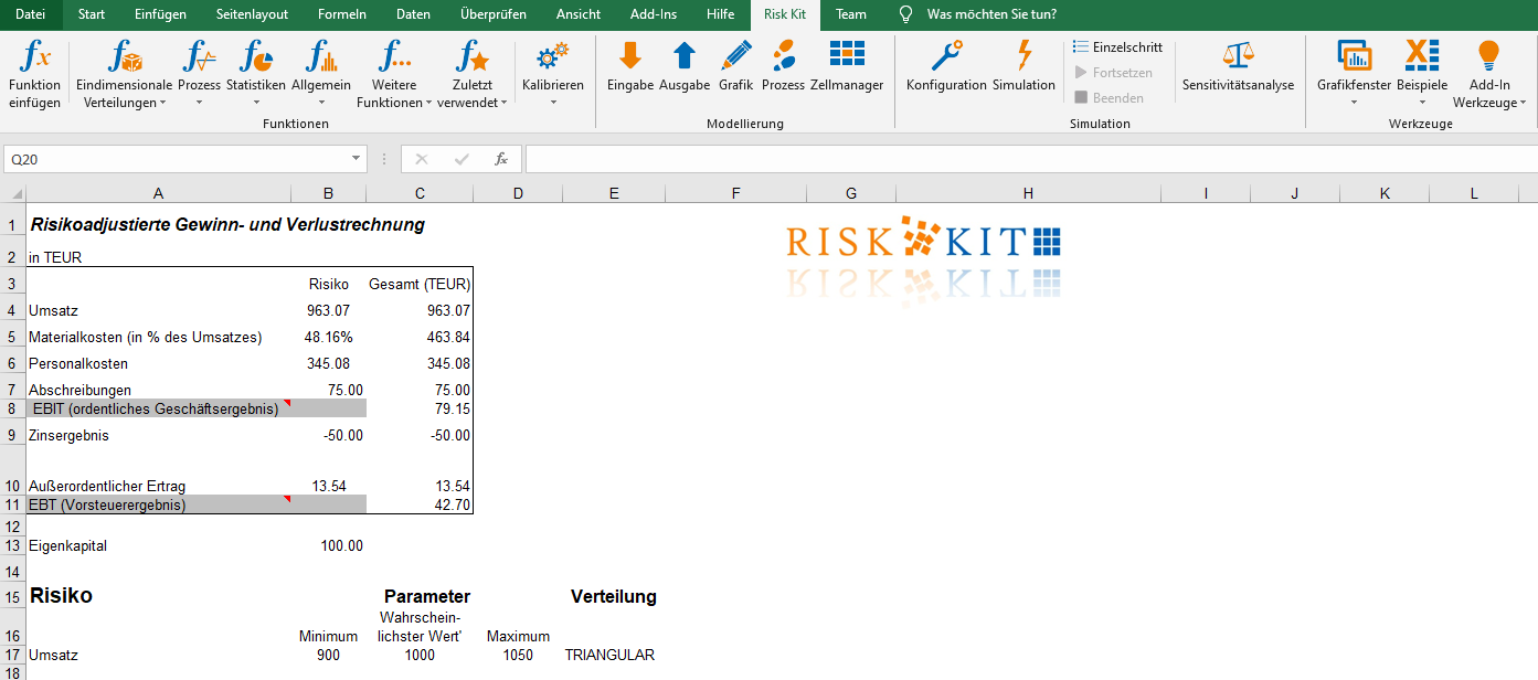
Figure 4: Modeling the revenue fluctuations.

To insert a triangularly distributed random number into the model, we select cell B4 and click the 'Functions' button on the Risk Kit ribbon.

This dialog box appears:

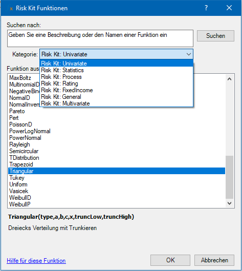
Figure 5: Function dialog box.

Risk Kit offers more than 430 functions from 7 categories:

1. Univariate: univariate, that is, one-dimensional probability distributions;
2. Multivariate: multivariate, that is, multidimensional probability distributions. This list contains functions that provide random numbers from multivariate distributions and copula functions;
3. Process: trends and random paths, and in some cases pointwise confidence bands, of stochastic processes;
4. Statistics: functions for calculating statistics of the simulated distributions, such as mean, variance, quantiles, and others;
5. General: this category contains functions for plotting arbitrary probability distributions and stochastic processes, for dynamic sorting, for calculating statistics of simulation results, for portfolio optimization and calculating the efficient frontier, and for designing delta-gamma engines;
6. FixedIncome: offers a range of basic functionality for interest rate instruments, such as handling interest rate and spread curves, calculating forward rates, calculating cash flows for interest-bearing transactions such as loans and bonds, valuing floating and fixed rate bonds, and calculating default probabilities from bond spreads;
7. Rating: rating functions for small and medium-sized enterprises in Germany, Austria, and the United States.

Since we want to insert a triangularly distributed random number, we select the category 'Univariate' and, in the list, the entry Triangular.

After we confirm the selection with 'OK', six functions are displayed:

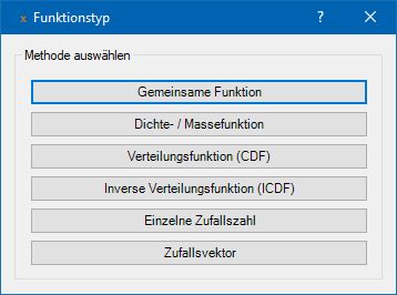
Figure 6: Functions for univariate distributions.

1. A common function in which the function type can be selected via a parameter.
2. The probability density function (PDF) for continuous distributions, or the probability mass function (PMF) for discrete distributions.
3. The cumulative distribution function (CDF),
4. The inverse cumulative distribution function (ICDF), and
5. A single random number (variate) of the distribution in question.
6. A vector of random numbers from the distribution in question. This function can be used for high-speed simulations when a model contains many risk factors from the same distribution family.

These functions are available for every one-dimensional distribution.

An alternative, and often more intuitive, way to select a distribution is to click the 'Univariate' button on the ribbon to open the distribution gallery.

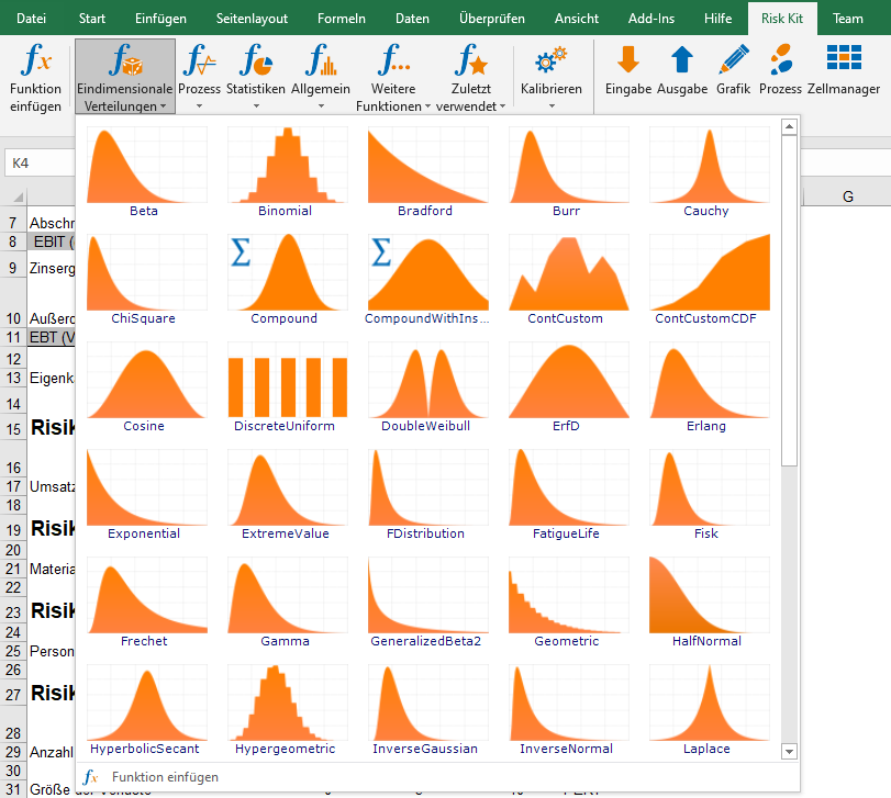
Figure 7: Distribution gallery.

The gallery shows a preview icon for each distribution that illustrates a typical shape of the distribution's density or mass function. The distributions are also sorted by name.

Move the mouse pointer over a preview icon to get more information about the distribution. A keyboard shortcut for the distribution is also displayed if one has been defined2.

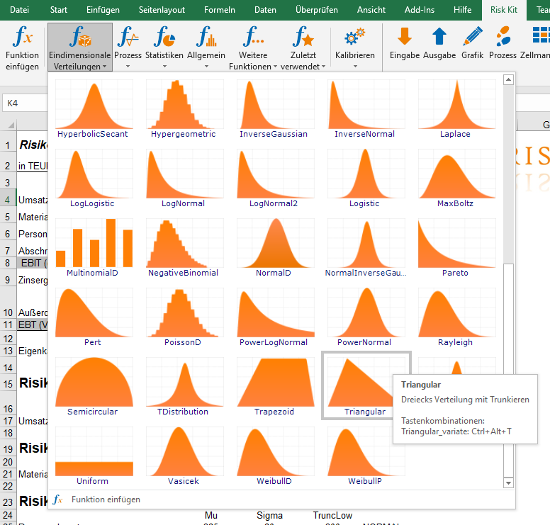
Figure 8: Information about the distribution and keyboard shortcuts in the gallery.

Click a distribution to select it from the gallery, and choose 'Single Random Number' as described above.

You can now enter the distribution parameters.

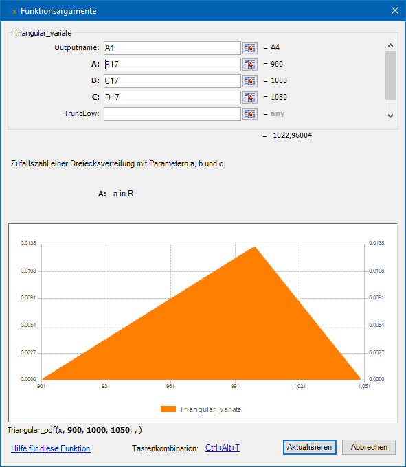
Figure 9: Function arguments of the triangular distribution.

There are two ways to do this. First, you can write the parameters into an Excel worksheet and specify a reference to the relevant cells in the function call. This is shown in Figure 9: Parameter 'a' contains a reference to cell B17 with the lower bound for revenue, 'b' contains a reference to C17 with the 'most likely value', and 'c' to D17, the most optimistic assumed revenue bound.

Alternatively, you can enter the parameters directly.

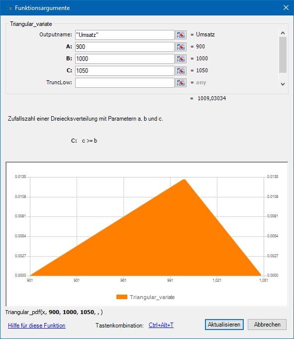
Figure 10: Function arguments.

In the dialog box, you can specify an output name (Outputname) (for univariate distributions only). The output name will appear in charts and statistics output as the legend for this distribution.

The dialog box also shows some further information about the selected distribution and its parameters. First, you get a brief summary of what the distribution does. In this case, it generates a 'random number from a triangular distribution with parameters a, b, and c'.

When you enter a parameter, information about its domain is displayed. In our case, it is required, for example, that parameter c be greater than or equal to b.

Below the chart, you see the definition of the function that is shown in the chart.

Finally, note the link to the online help in the lower left corner of the dialog box, and the function's keyboard shortcut at the bottom center.

When you click 'Insert', the function definition is entered into cell B4 and appears in Excel's formula bar. Total revenue in C4 now also reflects the risk. Material costs are affected by this as well, even though their percentage is still constant at 50%, because they also depend on revenue.

You can manually redraw random numbers by pressing <F9>.

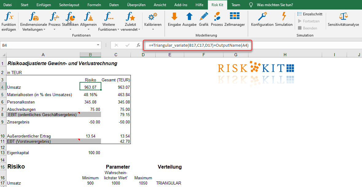
Figure 11: Cell containing the Risk Kit function.

We proceed similarly with the other risks. For the relative deviation from the planned material costs, we assume a normal distribution with expected value mu = 50% and standard deviation sigma = 3%.

Figure 12: Model assumptions for material costs.

To enter the formula in cell B5, we place the cursor on this cell and open the Risk Kit function dialog box. In the 'Search for' field, we enter 'normal' and confirm with 'Search'. When we select a function, we get a brief explanation of its meaning. This is how we determine that the function 'NormalD' is what we are looking for, namely, the normal distribution.

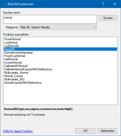
Figure 13: The function search dialog box.

We confirm the selection with 'OK' and choose 'Single Random Number'. This brings us to the dialog box in which we can enter the reference to B21 for mu and to C21 for sigma. Clicking 'Insert' enters the function definition into B5. Note that you can shorten this process by entering the function definition directly into the cell. The function dialog box is only there to help.

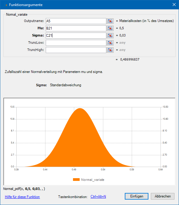
Figure 14: Function arguments of the normal distribution.

The absolute material costs are then the simulated costs as a % of revenue multiplied by the simulated revenue.

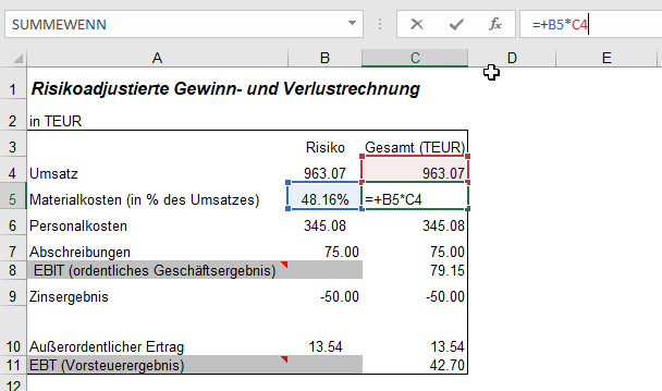
Figure 15: Linking the simulated material costs to the model.

We represent personnel costs similarly to material costs. We assume a normal distribution with expected value mu = 325 and standard deviation sigma = 20. However, we assume that personnel costs cannot fall below a certain level. We therefore assume that they are truncated on the left at 300.

Figure 16: Model assumptions for personnel costs.

To turn these assumptions into a function call, we open the function dialog box and link the parameters mu, sigma, and TruncLow to cells B25, C25, and D25.

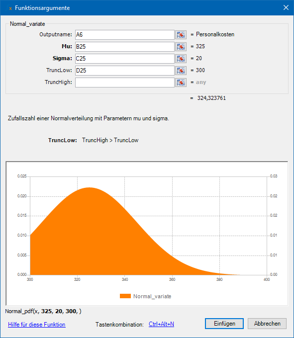
Figure 17: Normal distribution with truncation.

Truncating the distribution at 300 ensures that no random numbers below this value are drawn, while the distribution remains unchanged on the right side.

Clicking 'Insert' transfers the function into the worksheet

Finally, our company's extraordinary income is affected by credit risks. If customers default before invoices are paid, the company loses money.

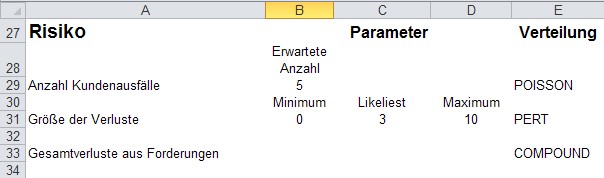
Figure 18: Model assumptions for extraordinary income.

We assume that the number of customers who default in the fiscal year is Poisson-distributed with an expected value of 5 defaults. If one or more defaults occur, we further assume that the size of each default is PERT-distributed, with a minimum loss of 0, a maximum loss of 10, and a 'most likely' loss of 3.

Note that we therefore have two sources of uncertainty at this point. First, the number of defaults is random, and second, so is the size of the loss in each individual case. The total loss is thus the sum of a random number of terms, each of which has a random amount.

We use the function dialog box to find out that the call for a Poisson-distributed random number reads

Poisson_variate(5)

and that the call for a PERT-distributed random number reads

Pert_variate(0, 3, 5).

Simple calls to these functions do not account for the fact that the losses differ in each individual customer default (the size of the terms). It is therefore not enough to draw a single Poisson-distributed and a single PERT-distributed random number and multiply them together, since this representation would imply that the losses are exactly the same size in every individual case.

To calculate the sum of a random number of terms, each of a random size, Risk Kit provides the function 'Compound'. Open the function dialog box, select 'Compound' from the gallery, and insert the function calls above as arguments.

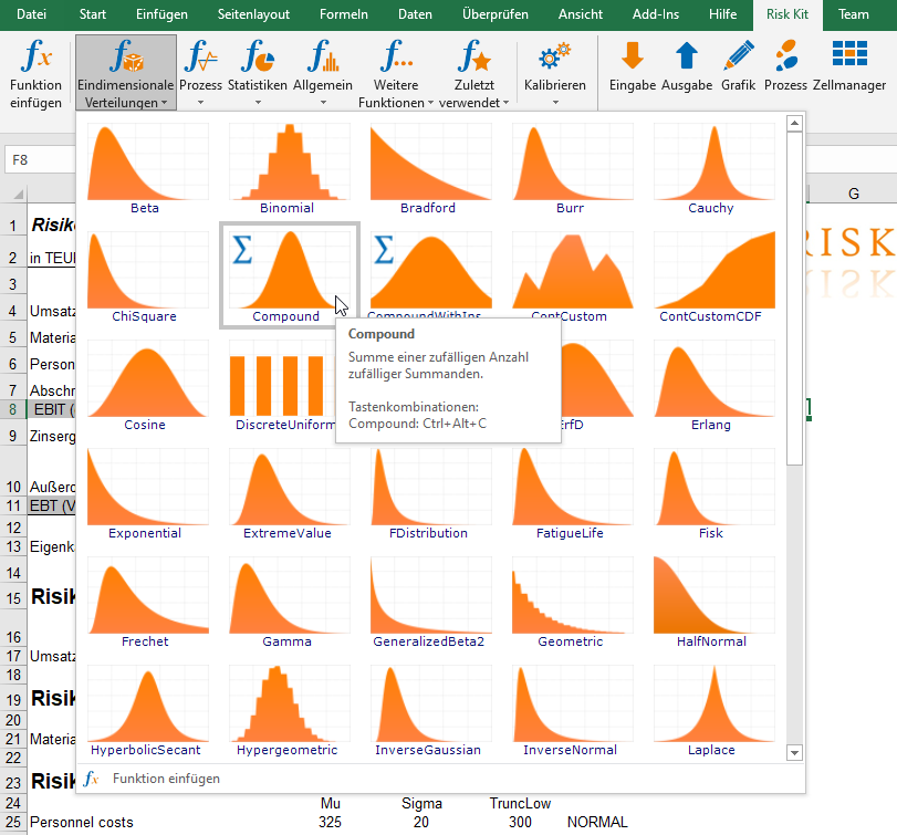
Figure 19: Compound distribution in the distribution gallery3.

The second parameter for the size of the losses must be entered in quotation marks to prevent Excel from evaluating the function immediately. The three parameters of the PERT distribution are then entered as Arg1 through Arg3.

Arg4 through Arg8 can be left empty. They are placeholders for other loss distributions with more than 3 parameters.

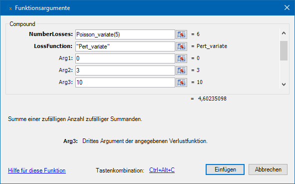
Figure 20: Calling the Compound function.

By confirming with 'Insert', we obtain the now fully specified model.

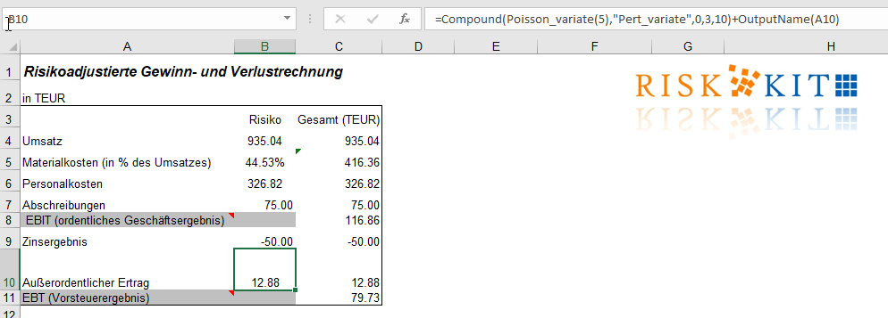
Figure 21: The fully specified model.

3.3. Defining the Model Outputs

Although the model is specified, we cannot yet run the simulation, because no model results have been defined yet.

As in the deterministic model, we are specifically interested in the behavior of EBIT and EBT under the influence of uncertainty. We therefore choose these quantities as model results (outputs). To do this, we select cell C8 and click 'Output' on the Risk Kit ribbon.

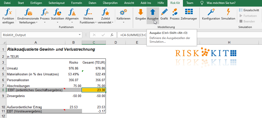
Figure 22: Defining output cells.

Cell C8 is now colored orange to visibly mark it as an output cell. You can also give output cells a name by adding the function '+OutputName("MyName")'. The name given in this way is used as the legend for the output cell in plots and other outputs.

We proceed in the same way for EBT in C11.

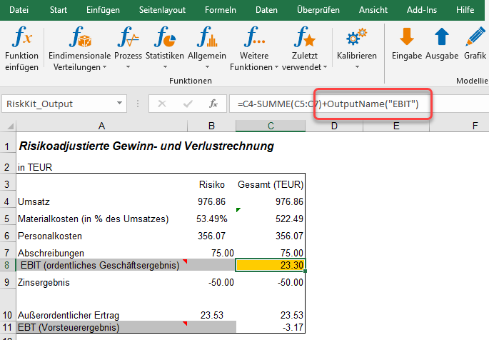
Figure 23: The OutputName function.

3.4. Configuring the Simulation

We are now ready to run the simulation. Open the configuration dialog box via the Risk Kit ribbon to set the number of simulation runs. 5,000 runs are selected as the default. The screen is updated every 500 runs.

Figure 24: Opening the configuration dialog box.

In the configuration dialog box, you can enable 'Output Default Statistics' to get an overview of the statistics of the simulated distributions displayed on a new 'Output' worksheet once the simulation has finished. If you select 'Output Simulation Results', the results of every single simulation run are output on another worksheet.

'Generate Charts' displays the distributions in the output cells graphically, provided plots have been defined (see below). If you enable 'Online Charts', the chart functions are redrawn every time the screen updates, so you can watch the output distributions develop. If 'Plot All Output Cells' is enabled, all output cells are plotted without having to specify plot functions explicitly.

If you check 'Reset Seed', the seed of the random number generator is reset to its original value at the start of the simulation, so that identical sequences of random numbers are generated across different simulations.

If 'Insert Function Definition as Comment' is enabled, the cell's function definition is attached as a comment every time you use the Risk Kit function dialog box.

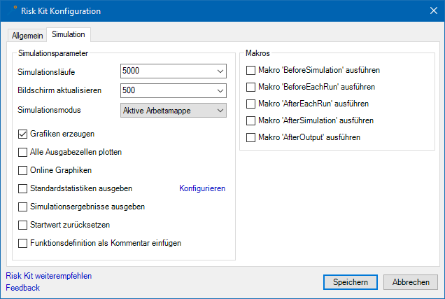
Figure 25: Configuration dialog box.

Select the scope of the simulation from the dropdown list in the configuration dialog box. If your model is on a single worksheet, select 'Active Worksheet'. In this case, the worksheet containing the model must be active when the simulation is started. This option is set as the default. Risk Kit additionally offers the options 'Active Workbook' and 'All Open Workbooks', which must be used when a model is spread across multiple worksheets in a workbook, or even extends across multiple workbooks. We select 'Active Workbook', since we will add result statistics on additional worksheets later.

Risk Kit lets you write your own macros and have them run during the simulation. This allows you to update input values before the simulation, save intermediate results, and so on. In the configuration dialog box, specify which macros you want to run, and at which point in the processing. Note that the macros must be located in the active workbook and have exactly the specified name. If

1. 'Run Macro BeforeSimulation' is checked, the macro named 'BeforeSimulation' is executed before the simulation starts.
2. 'Run Macro BeforeEachRun' is checked, the corresponding macro is executed before each simulation run.
3. 'Run Macro AfterEachRun' is checked, the corresponding macro is executed after each simulation run.
4. 'Run Macro AfterSimulation' is checked, the corresponding macro is executed at the end of the simulation.
5. 'Run Macro AfterOutput' is checked, the corresponding macro is executed after the output of statistics and simulation results (see above).

Enable 'Output Default Statistics' and confirm with 'Save' to close the configuration dialog box.

3.5. Running the Simulation

Figure 26: Starting the simulation.

Now that the simulation is configured, you can start it. To do so, click 'Simulate' on the ribbon.

During the simulation, the number of runs already completed is displayed in Excel's status bar in the lower left corner of the screen.

Figure 27: Status information.

You can cancel the simulation with <CTRL><T>.

If you pause the simulation with <PAUSE>, you can resume or end it using the corresponding buttons on the ribbon.

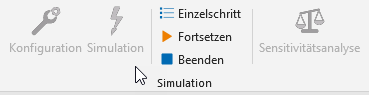
Figure 28: Canceling the simulation.

Risk Kit lets you run the simulation step by step. After each single step is performed, the simulation pauses.

After the simulation, a new 'Output' worksheet is appended to the active workbook. This sheet contains a column of default statistics for each output cell of the simulation. The heading used is the specified output name, or the cell address if no name was specified.

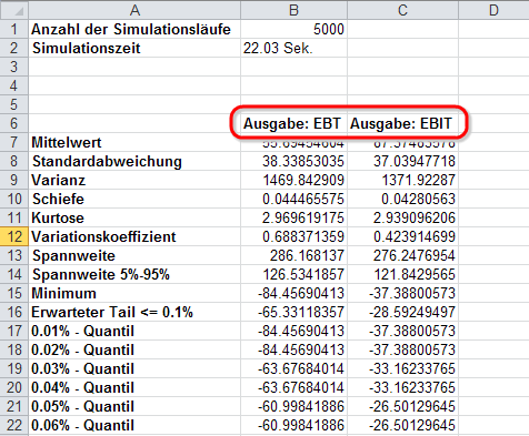
Figure 29: Output statistics.

Similarly, you can have all the random results for the output cells output if you enable the 'Output Simulation Results' option in the configuration dialog box.

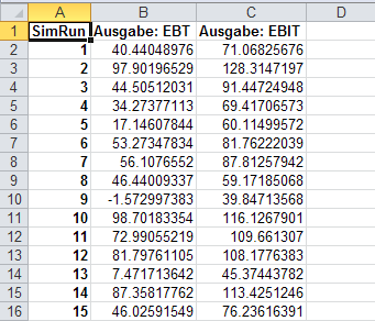
Figure 30: All simulation results.

4. Charts

To get an impression of the shape of the EBIT and EBT distributions, as well as of the risk factors that go into the model, you can extend the model with charts by displaying charts in cells or inserting a chart function into the worksheet.

The simplest way to visualize a distribution is to click 'Configuration' on the Risk Kit ribbon and enable the 'Show Histograms in Cell' checkbox. After a simulation, a histogram of the relevant distribution is then displayed in every output cell without having to enter any further functions. So you can mark any cell whose distribution you want to see as an output cell, and you get the visualization after rerunning the simulation.

Additionally, enable the 'Online Charts' checkbox to watch the distribution develop during the simulation.

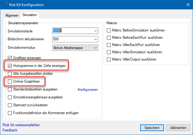
Figure 31: Displaying histograms in all output cells.

If you only want to display charts for individual outputs, you can do this with the function 'PlotInCell'. For this, it is not necessary to enable the checkbox mentioned above. Simply append the function 'PlotInCell' to the formula in a cell, analogous to the function 'Outputname'. The function returns the value 0, so it does not change the result of the formula. As its only required parameter, the function references the output cell whose distribution is to be displayed. The function can, but does not have to, itself be located in an output cell.

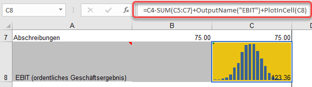
Figure 32: The 'PlotInCell' function.

The function has two more parameters.

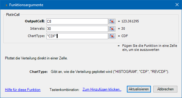
Figure 33: Parameters of the 'PlotInCell' function.

They let you specify exactly the number of intervals in the display (the default is 20) and set the type of chart (histogram, distribution function, or reverse distribution function; the default is "HISTOGRAM". Note the quotation marks.).

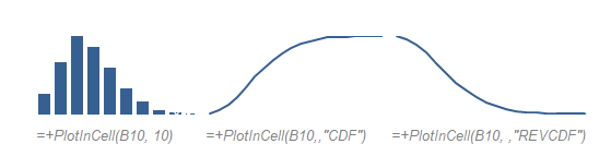
Figure 34: Various outputs of the 'PlotInCell' function.

If necessary, set the font color for the cells in which a distribution is shown to match the background color, white in the example above, to make the value 0.0 returned by the function invisible.

The second way to visualize is provided by the function 'Plot'. This function calculates and draws a histogram of the specified simulated distribution, along with its cumulative distribution function (CDF) and inverse and reverse cumulative distribution functions (ICDF, reverse CDF); it also estimates its kernel density and draws a box plot.

The Plot function can include numerous optional arguments, such as legends, the title, and the option to embed the chart in a worksheet. You will find detailed information on all the particulars of the Plot function in the online help.

You will find the Plot function in the function dialog box in the category 'General'.

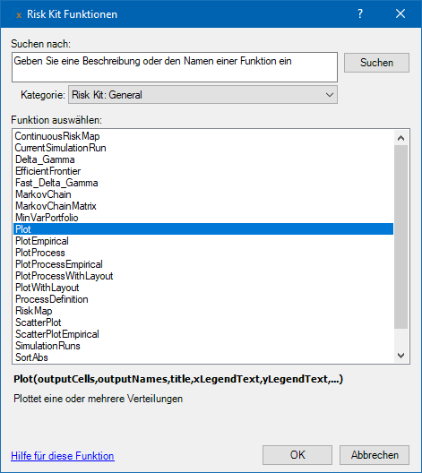
Figure 35: General functions.

The dialog box guides you through the function parameters.

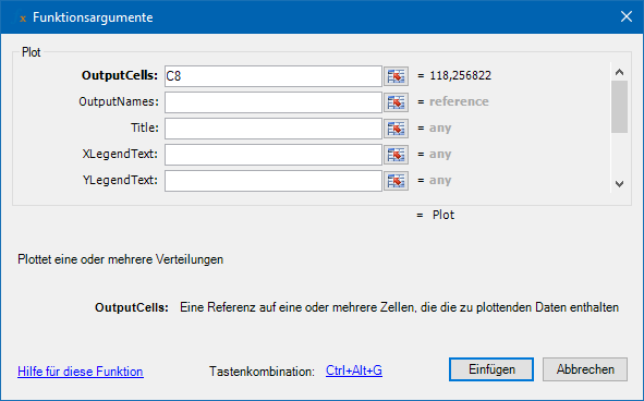
Figure 36: Defining the Plot function.

The only non-optional parameter of the Plot function is a reference to an output cell of the simulation. This means you can generate charts very easily, for example, by writing '+Plot(C8)' into an empty cell4.

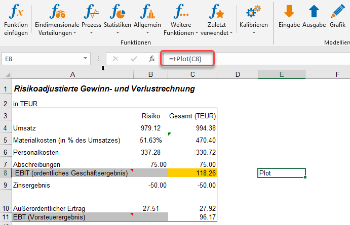
Figure 37: The Plot function.

Note that two requirements must be met for a Plot function to be executed. First, the cell containing the function must be marked as a chart cell via the ribbon. In this case, the cell turns dark orange.

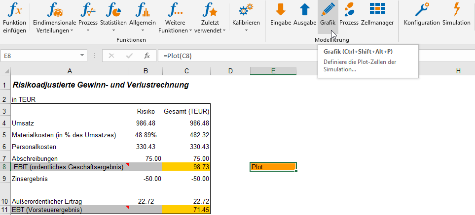
Figure 38: Marking a cell as a chart cell.

Second, the 'Generate Charts' checkbox must be checked in the configuration dialog box.

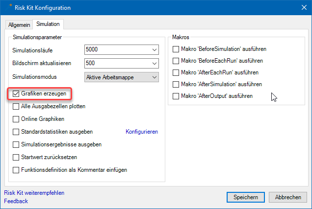
Figure 39: Configuration dialog box.

After the simulation is restarted, the chart is generated.

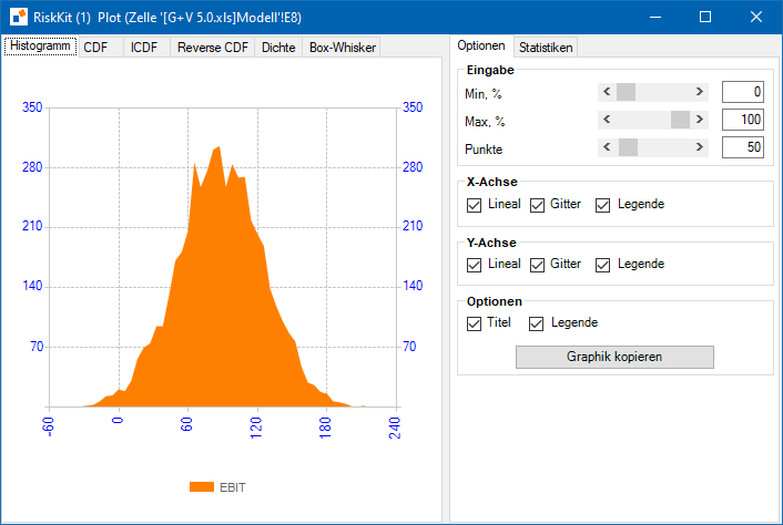
Figure 40: Chart window.

The output cell's output name 'EBIT' is used as the legend for the distribution. Note that right-clicking the chart, the legend, and so on gives you access to an extensive context menu that lets you customize the chart's layout, as well as colors, fonts, scaling, styles, and many other settings.

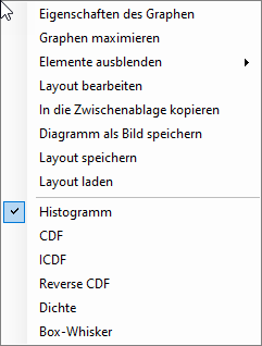
Figure 41: The chart's context menu.

The axis properties dialog box lets you set the number of decimal places displayed, as well as the display of a thousands separator, a unit and its label (for example, TEUR), the number of labels displayed, and so on.

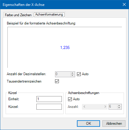
Figure 42: Properties of the left Y axis.

You can switch between histogram, CDF, ICDF, and reverse CDF with <CTRL>-D, or by clicking the corresponding tabs, or via the context menu (see Figure 37).

Using the controls on the right side of the plot window, you can customize the appearance of the plot:

• You can change the displayed value range, that is, the smallest and largest quantile between which the distribution is plotted. If several distributions are shown in one chart, the displayed value range extends from the smallest lower quantile to the largest upper quantile of these distributions.
• Enable the checkboxes to show the ruler and the grid for the x and y axes.
• Select the discretization of the x axis (points).
• Enable the checkboxes to show the legend for the x and y axes.
• Copy the chart to the clipboard so you can paste it into other documents.
• Enable the checkbox to display the title or the legend.

On the right side of the window, you will find the 'Statistics' tab with default statistics. Double-clicking a row of the table displays that statistic in the chart (Figure 39). Double-clicking the heading of a column removes the corresponding distribution from the chart, or shows it again. This is especially helpful when you have several distributions shown in one chart.

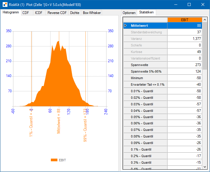
Figure 43: Statistics as part of the chart.

Risk Kit provides three different options for scaling the y axis:

1. Density function: the vertical axis is scaled so that the area under the histogram equals 1;
2. Relative frequency: the vertical axis is scaled so that it represents the relative frequency of the realizations in a bar of the histogram;
3. Absolute frequency: the vertical axis shows the absolute frequency of the simulation results in a bar of the histogram.

Open the context menu of the left y axis to select the scaling.

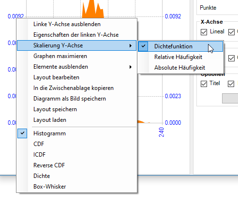
Figure 44: Scaling the y axis.

You can copy the chart to the clipboard via the context menu to paste it into your presentations.

If you want to embed the chart into a worksheet after the simulation, specify the parameters outputChartCell and outputChartType in the Plot function (see Figure 41). The first parameter specifies the cell into which the top-left corner of the chart is inserted. The second parameter defines how the distribution is displayed. In the example, the distribution is plotted as a histogram. You can also specify the width and height of the chart in pixels.

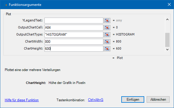
Figure 45: Defining the Plot function.

Confirm with 'Insert' to insert or update the function in the cell.

After the simulation, the plot is embedded in the worksheet.

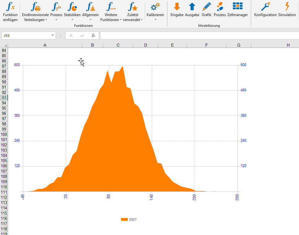
Figure 46: Embedded chart.

Risk Kit automatically replaces the embedded charts after every rerun of the simulation.

Risk Kit lets you delete all embedded charts and all chart windows by selecting the corresponding menu item 'Close Chart Windows' from the dropdown menu on the ribbon.

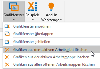
Figure 47: Dropdown menu of the 'Chart Windows' button.

This only deletes the charts that were inserted by Risk Kit itself. All other charts remain unaffected.

4.1. Statistics Functions

Risk Kit provides cell functions that let you query result statistics in worksheets, so that formatted reports can be created. You will find these functions in the category 'Statistics' of the function dialog box.

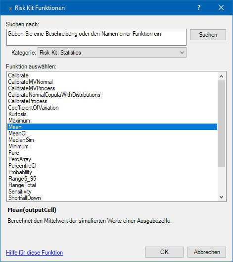
Figure 48: Statistics functions.

This category contains functions such as:

• Maximum: calculates the maximum of the simulated values of an output cell;
• Mean: calculates the mean of the simulated values of an output cell;
• MedianSim: calculates the median of the simulated values of an output cell;
• Minimum: calculates the minimum of the simulated values of an output cell;
• Range5-95: calculates the range between the 5% and 95% quantiles of the simulated values of an output cell;
• Variance: calculates the variance of the simulated values of an output cell;
• Perc: calculates a quantile, that is, the Value at Risk of an output cell at the specified confidence level;
• …

Place the cursor on an empty cell and select the Mean function from the category 'Statistics'. The dialog box for entering the function arguments appears:

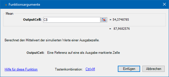
Figure 49: Defining the mean function.

The parameter OutputCell references cell C8, which defines a model result. Confirm with 'Insert' to insert the function into the active cell.

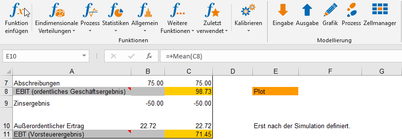
Figure 50: Mean function.

When the Mean function is defined, it returns the value 'Not defined until after the simulation'. The reason for this is that the distribution represented by the output cell is not known until the simulation has been run.

You can also place the result statistics on a different worksheet to create clear reports that summarize the simulation results. Such a report can contain statistics as well as embedded charts.

Note that you can define new risk and return measures by combining results with other quantities, such as RAROC as risk-adjusted return relative to capital, or mean EBT (at risk) relative to equity.

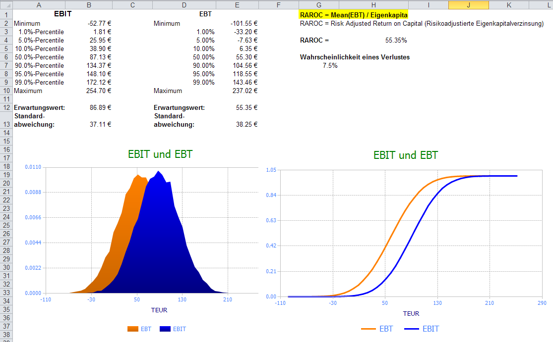
Figure 51: Results report.

5. Sensitivity Analyses

Sometimes it is of interest to see which random input parameters or intermediate results have the strongest effect on the model outputs. To perform such a sensitivity analysis, define all the cells whose effect you want to examine as input cells5. Select the cells with the values for revenue (B4), material costs (B5) and personnel costs (B6), and extraordinary income (B10), and click the 'Input' button on the Risk Kit ribbon (see Figure 52).

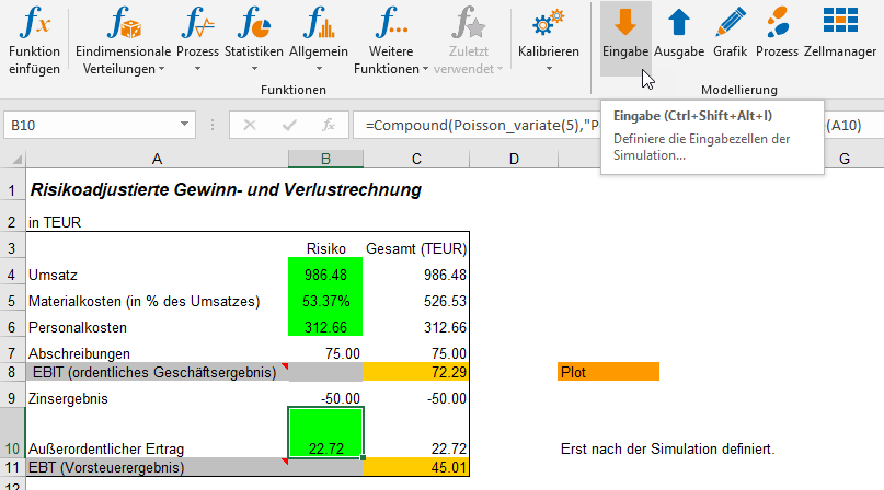
Figure 52: Defining the input cells.

These cells are now colored green to clearly mark them as input cells. Conversely, you must mark all the cells whose dependency on the input cells you want to analyze as output cells. Here, we consider EBIT and EBT, which have already been marked as output cells.

Note that it is not necessary for the input cells to contain random numbers that are drawn directly in every simulation run. They can instead also contain intermediate results of the simulation that still depend on other cells.

Once all input cells have been defined, click the 'Sensitivities' button on the Risk Kit ribbon.

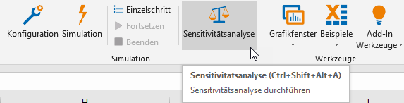
Figure 53: Opening the sensitivity analysis dialog box.

The following dialog box appears:

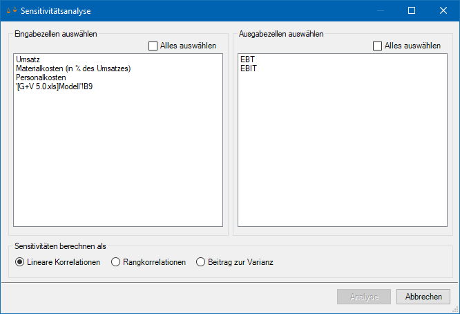
Figure 54: Sensitivity analysis.

Select all the input and output cells from the lists that you want to include in the analysis. Specify the sensitivity type, for example, 'Linear Correlations'. The sensitivities are then calculated as linear correlations, that is, using the Pearson correlation coefficient. Start the calculation by clicking the 'Analyze' button.

After the simulation is complete, Risk Kit displays the results in the following dialog box:

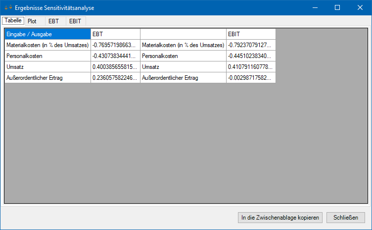
Figure 55: Results of the sensitivity analysis.

By clicking the 'Copy to Clipboard' button, you can copy the results and paste them into a worksheet with <CTRL>-<V>.

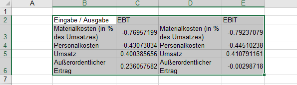
Figure 56: Sensitivity analysis results in a worksheet.

The sensitivities are displayed in an overview chart and in an individual chart for each output cell. You can switch between the charts by clicking the corresponding tabs.

You can read directly from the chart that, in our example, material costs have the strongest effect on EBT. In particular, an increase in material costs leads to a decline in EBT. This intuitive fact is reflected by the negative sign of the sensitivity.

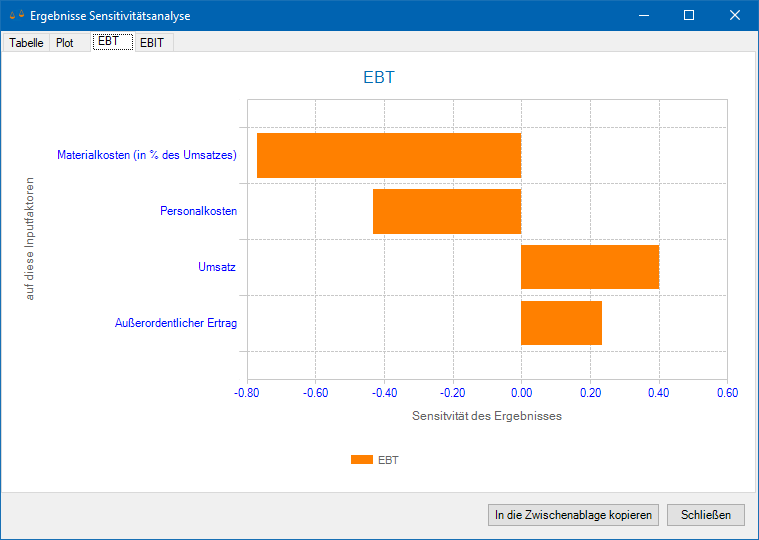
Figure 57: Results chart of the sensitivity analysis.

5.1. Sensitivity Analyses with the Risk Kit Cell Function

Risk Kit provides a cell function, Sensitivity, that lets you perform the same sensitivity analyses as with the analysis dialog box described above. When using the cell function, however, the results can be embedded in a worksheet and run together with the simulation. The function is located in the category 'Statistics' of the function dialog box (see Figure 58Error: Reference not found).

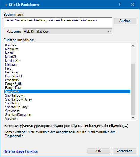
Figure 58: The Sensitivity cell function.

Go to an empty cell and select the function Sensitivity from the function dialog box. The input dialog box shown in Figure 59Error: Reference not found appears

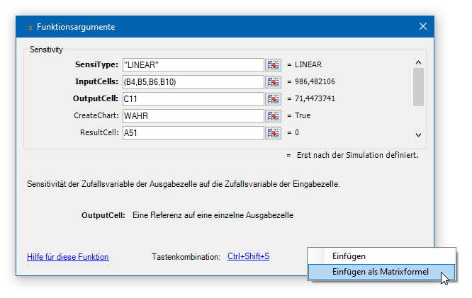
Figure 59: Defining the Sensitivity function.

The parameter sensiType = "LINEAR" specifies that the sensitivities are calculated as linear correlations. The parameter InputCells refers to cells B4, B5, B6, and B10 on the worksheet 'Model'. The parameter OutputCell refers to output cell C11 on the worksheet 'Model' (EBT in our example).

Set the parameter CreateChart to TRUE if you want to embed result charts into a worksheet after the simulation. The parameter ResultCell specifies the cell into which the chart is embedded (cell A51 on the worksheet 'Sensis').

Since the sensitivity function returns an entire table as its result instead of a single number, it is an array function in Excel. To enter it as such, select "Insert as Array Formula" from the dropdown list6.

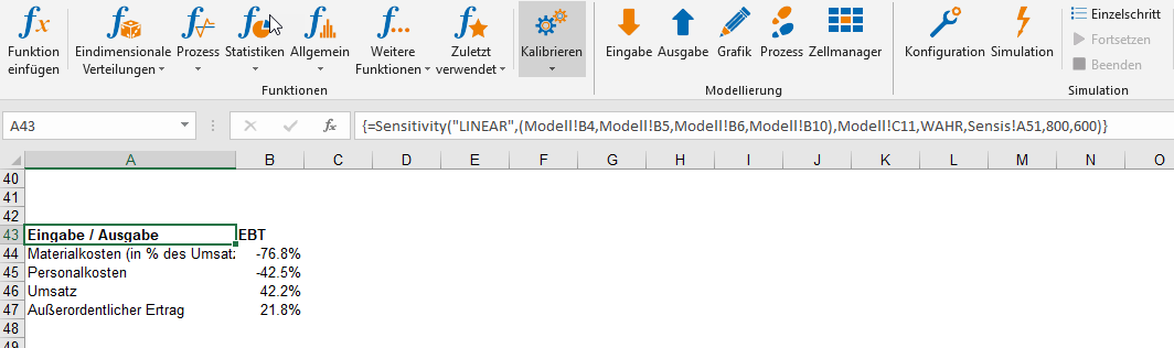
Figure 60: The Sensitivity function.

The formula now appears in curly braces in Excel's formula bar (see Figure 60Error: Reference not found).

Once the Sensitivity function is defined, click the 'Simulate' button on the Risk Kit ribbon to start the simulation. The sensitivities are displayed after the simulation. You can format the results like any other Excel cell.

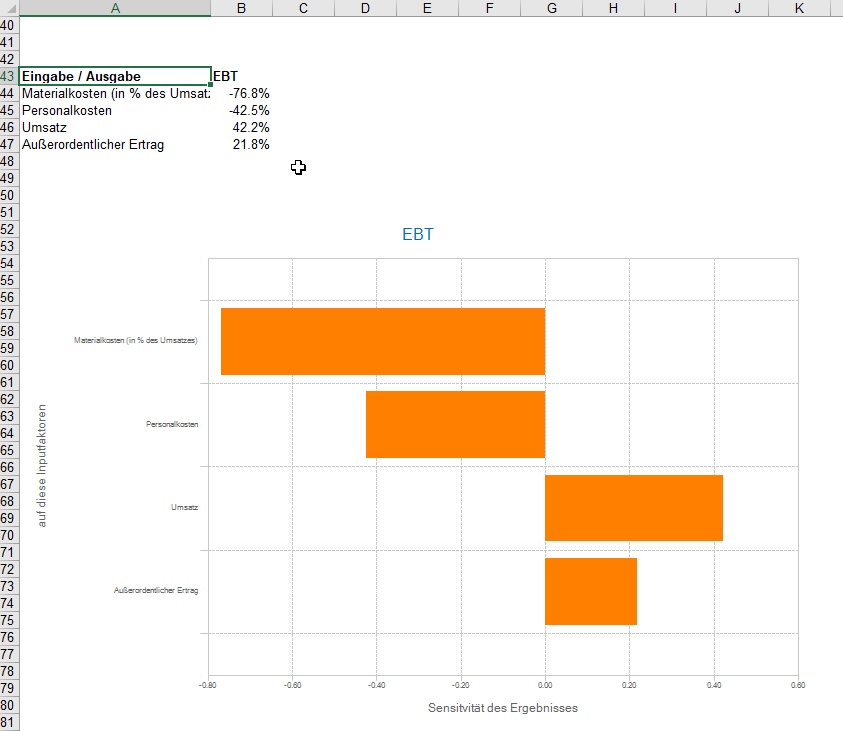
Figure 61: Sensitivity analysis results.

6. Summary

Monte Carlo simulations offer a high degree of flexibility in building and solving risk models of almost any complexity. Risk Kit supports the modeling and analysis process and significantly reduces the time and cost involved in Monte Carlo simulations. Risk Kit is easy to use and fits into your familiar working environment.

Beyond the functionality shown in this example application, Risk Kit offers one- and multidimensional stochastic processes, multidimensional distributions and copulas, as well as parameter estimation for distributions.

Risk Kit is available with a single-user license (Professional) and with a network floating license (Enterprise). A free, renewable license for a single-user version with a reduced feature set (Light), but licensed for commercial use, can be obtained online at license.wehrspohn.info.

Please contact us for more information.

7. Our Products

The Risk Kit suite is integrated into Excel and extends the risk manager's workspace with all the functions of modern risk management.

Risk Kit

• Monte Carlo simulation with all practically relevant one- and multidimensional distributions
• Simulation of developments
• Visualization of risks
• Reporting
• Calibration

Risk Kit R

• Statistical analyses with R

Risk Kit Data

• Online market data connectivity to the European Central Bank, Federal Reserve Economic Data, the World Bank, Eurostat, and Marketstack
• Exchange rates, interest rate curves, commodity prices, stock prices, economic and social statistics

The Risk Kit suite is available in single-user and enterprise licenses.

The Enterprise Risk Evaluator is a central platform for the company-wide risk management process. It offers

• Qualitative and quantitative risk identification and assessment.
• Risk aggregation, risk-bearing capacity, risk analysis
• Integration with planning
• User-definable reporting
• Measure controlling and internal control system
• Incident and loss management

The Enterprise Risk Evaluator can be combined with the Risk Kit suite.

The Market Risk Evaluator is a system for market risk analysis for banks. It includes

• Market data imports and consolidation
• Cash flow calculations
• Sensitivity calculations
• Scenario analyses
• Monte Carlo simulation with various models
• Portfolio and market factor backtesting

The Credit Risk Evaluator is a tool for credit portfolio analysis, also for banks. It offers

• Several portfolio models, including CreditMetrics and CreditRisk+
• Single- and multi-period models
• Risk and return analyses
• Country risks
• Drill-down to any level of segmentation, from the individual transaction to the bank as a whole

In addition to our products, we offer consulting services, in particular on

• Model design
• Risk management methodology
• Business process design
• Risk analyses
• Integration of our systems
• Development of client systems
• Training

Please get in touch with us if you would like more information or a web-based presentation.

1 You can download the example model as well as the Risk Kit software in the login area. You can choose your own username and password.

2 To add or delete keyboard shortcuts, click "Add-in Tools: Keyboard Shortcuts" on the ribbon.

3 Note the second version of the compound distribution, which also includes insurance thresholds.

4 You can plot several distributions at the same time by entering the references to the distributions' output cells in parentheses, for example, '+Plot((C8,C11))', to make it clear to Excel that (C8,C11) represents the value of the first parameter of the Plot function.

5 You can mark the same cell as both an input cell and an output cell at the same time. In particular, this means you can also apply the function 'PlotInCell' to cells that are marked as input cells.

6 Note that in Excel, you can also enter an array formula manually by selecting the entire result range, clicking in the formula bar, and pressing <CTRL><SHIFT><ENTER>.