
Introducing Risk Kit Data
Risk Kit Data is an add-in for Microsoft Excel. Once installed, the add-in is available as a new ribbon.

Figure 1: The Risk Kit Data ribbon.
Risk Kit Data provides a graphical user interface for browsing statistics and financial data. Use the Finance task pane by clicking 'Browse Financial Data' in the ribbon to retrieve current and historical stock and index prices as well as exchange rates. Access the Data task pane by clicking 'Browse Historical Data' to browse the full databases of the European Central Bank (ECB), Eurostat, Federal Reserve Economic Data (FRED), the World Bank, and Apilayer Marketstack.
Use the examples under the 'Example Workbooks' dropdown menu to get started with Risk Kit Data. Under 'Add-in Info' you will find the online help as well as information about the add-in.
To disable the add-in in Excel, go to 'Add-in Settings' and click 'Disable Add-in'.
Note that you need a personal API token from Apilayer Marketstack to access their data feeds. To request a token, go to 'Add-in Settings' in the ribbon and follow the link shown there. You will also find a reference to the terms of use for the data there.
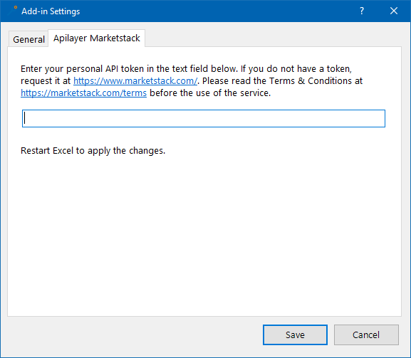
Figure 2: Add-in settings and API token
Profit and Loss Model
The oil price has changed significantly in recent years. This high volatility particularly affects companies that import crude oil and other commodities. In this section, we consider a profit and loss model in which the oil price is an important source of randomness. We also include the USD/EUR exchange rate and a 1-year EUR interest rate as additional examples of typical market factors. To obtain the historical prices for these factors and to consolidate the time series, we will use Risk Kit Data.
We will also use another add-in, Risk Kit, to estimate the parameters of process models for the data and to run a Monte Carlo simulation of the profit and loss model. For a detailed introduction to Risk Kit, see Wehrspohn/Zhilyakov, Monte Carlo Simulation with Risk Kit, 2021.
Defining the Model
As a first step, we define a simple, purely illustrative P&L model and identify its sources of randomness (Figure 3). To calculate gross profit and loss, we start with revenue (D7) and deduct all expenses, including material costs (D8), raw materials (D9), personnel costs (D10), and depreciation (D11). This leads to the intermediate result 'earnings before interest and taxes' (EBIT) (D12). We then calculate 'earnings before taxes' (EBT) (D15), which corresponds to the sum of interest income (D13) and extraordinary income (D14) added to EBIT.
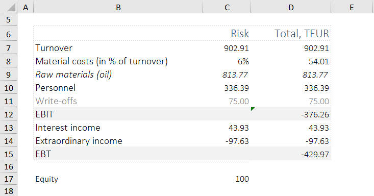
Figure 3: Profit and loss model.
Let us assume that revenue (C7), material costs (C8), raw materials (C9), personnel costs (C10), as well as interest (C13) and extraordinary income (C14) are subject to risk.
We assume that revenue (C7) has a triangular distribution with parameters a=900, b=1000, and c=1050, meaning that revenue fluctuates between 900 and 1050, with 1000 as the most likely value.
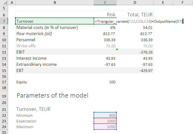
Figure 4: Identifying the sources of randomness.
You may also notice the function 'OutputName' in the formula bar, appended to the distribution. This function sets the label for this particular risk, which we will see later in the charts.
For material costs, we assume a normal distribution with mean = 4% and standard deviation = 2%.
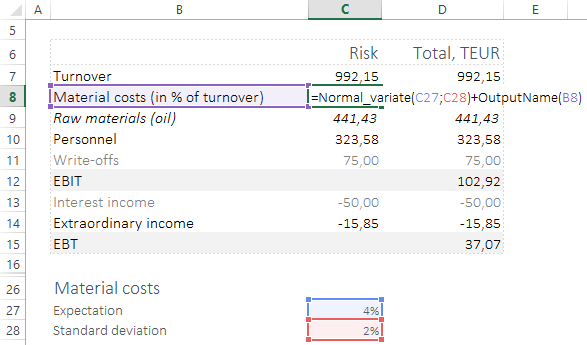
Figure 5: Identifying the distribution for material costs.
Since actual material costs are variable and depend on the level of revenue, we model them as a relative quantity, 'as a % of revenue'. The total material costs in D8 are therefore equal to the relative costs (C8) multiplied by total revenue (D7).
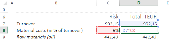
Figure 6: Calculating total material costs.
One of the largest expenses in our example is raw materials, which are the product of the total volume of imported oil (barrels) and its price. We assume that the volume of imported oil is uniformly distributed over the interval from 7.5 to 9.5 thousand barrels. To estimate the oil price, we analyze the historical market data.
Selecting the Data
To obtain the historical prices, click 'Browse Historical Data' in the Risk Kit Data ribbon (Figure 1). The add-in then opens the Data task pane.
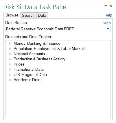
Figure 7: The Data task pane.
The Data task pane allows you to browse historical statistics from various data sources, run searches, filter and select data, and load the data into Excel.
To run a search, activate the Search tab (Figure 8), enter the search query in the text field, and press ENTER. In our example, we search for 'Crude Oil'. Note that the process can take a few minutes depending on the search query.
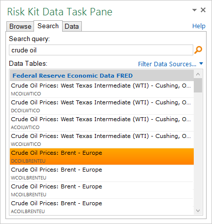
Figure 8: Browsing the data.
It is also possible to narrow the search by excluding results from some data sources. To do so, click 'Filter Data Sources' and clear the checkboxes for the data sources you want to exclude.
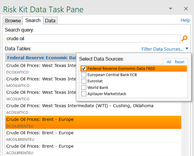
Figure 9: Filtering data sources.
We will use the historical prices for Brent crude oil for our estimates. Double-click the table 'Crude Oil Prices: Brent - Europe' in the list to load the historical data. You will notice that there are four similar tables in the search results. The difference between these tables lies in the frequency of the data. We use the first table, with daily frequency, which provides prices for business days.
After double-clicking, the add-in activates the 'Data' tab.
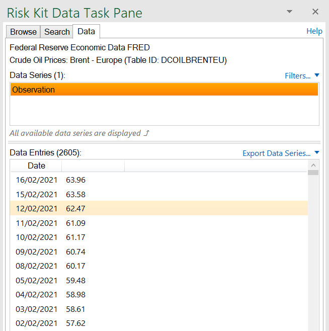
Figure 10: Loaded data series.
In this example, we use the Federal Reserve Economic Data source, which offers only one data series per table. The other data sources can have thousands of data series per table. Use the filters to reduce the number of data series and to set the time window of the observations (Figure 12).
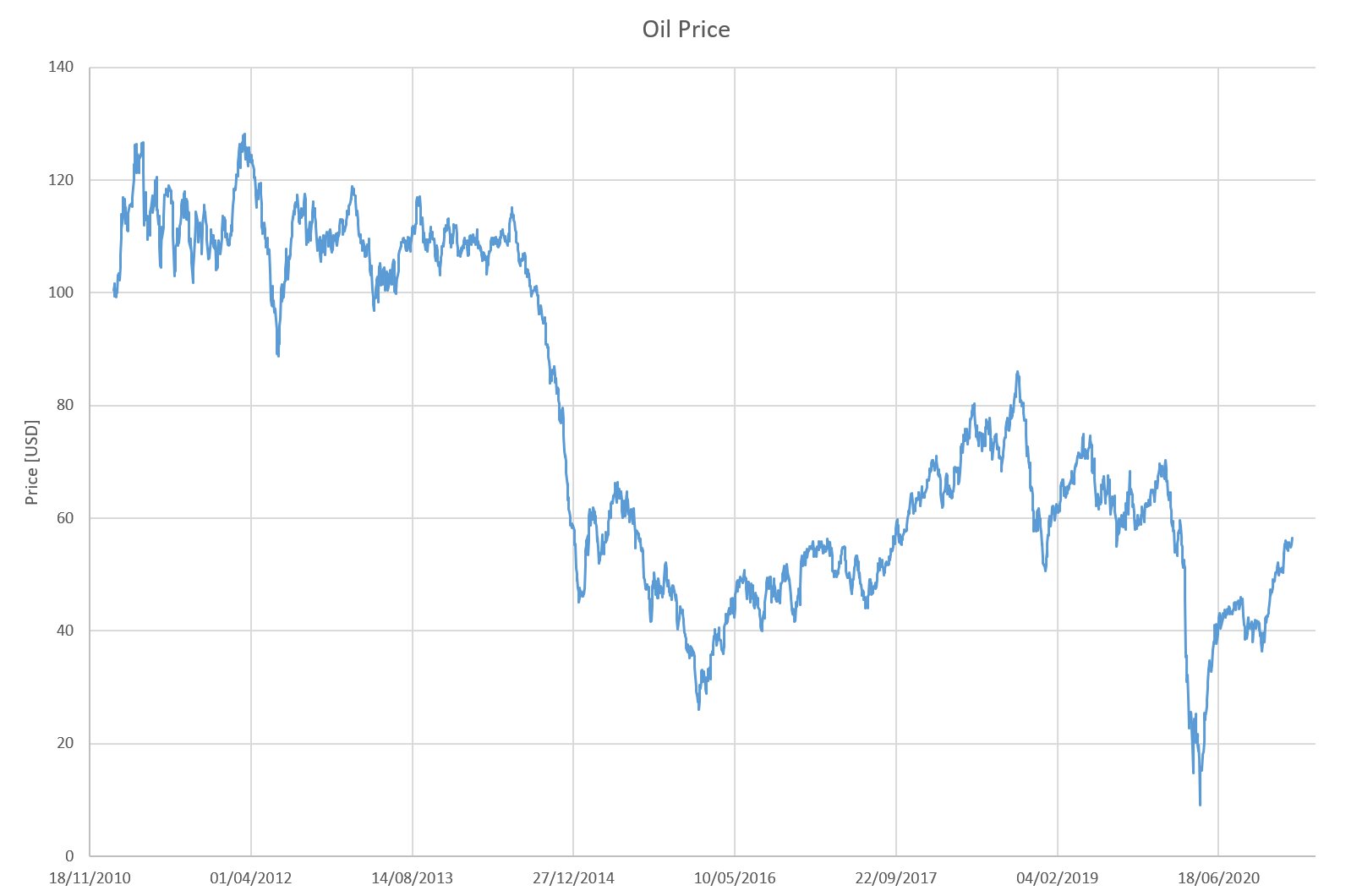
Figure 11: Oil price between 2011 and 2021
Oil prices have been quite volatile over the past ten years, ranging between 9.12 USD per barrel on April 21, 2020, and 128.14 on March 13, 2012. To obtain a more homogeneous sample that is representative of the current market situation, we therefore set the time window to the period from February 21, 2015, to February 21, 2021.
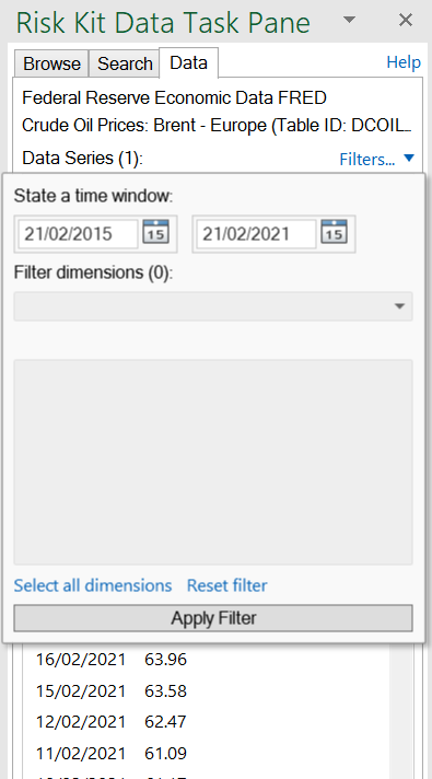
Figure 12: Filtering data series.
Click 'Apply Filter' to filter the data series.
If you hover the mouse pointer over the table name, you will see the detailed description in the tooltip. Note the units of the data.
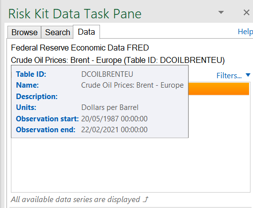
Figure 13: Description of the table.
To export the data into the worksheet, click 'Export Data Series'. The tool offers two options here. The data can be exported either as a cell function or as raw values. The cell function often offers more control over the data. In particular, it lets you sort the observations by date in ascending or descending order, retrieve several data series at once, change the time window afterward, and so on.
To output the series ID in the first row and the data in the first column, select the corresponding checkboxes.
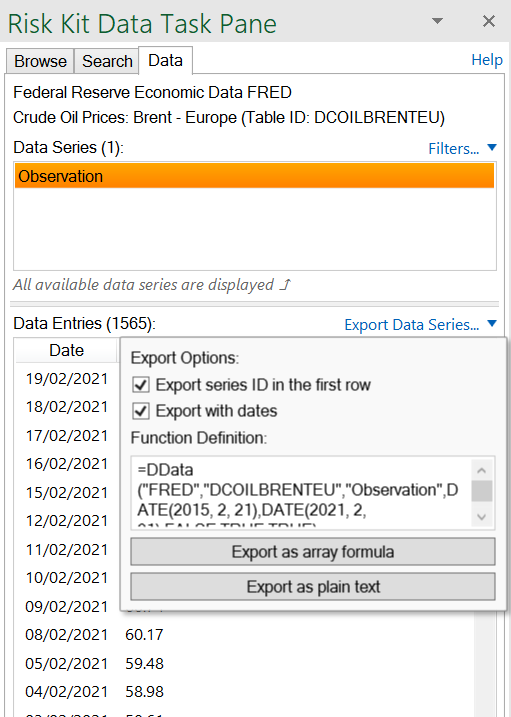
Figure 14: Exporting the data.
The add-in automatically fills the required number of rows and columns.
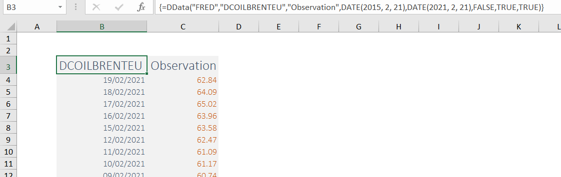
Figure 15: Example of the DData cell function.
To update the parameters of the function, you must either edit the function in the Excel formula bar or use the Risk Kit Data function dialog box. To do this, select a cell where you want to place the function, and click 'Insert Function' in the Risk Kit Data ribbon (Figure 1). In this particular example, we sort the observations in descending order by date, so that the most recent date has a stable position in the worksheet. This is often helpful, since later forecasts start from the most recently known value of a series.
To do this, we set the function's 'DatesInIncreasingOrder' argument to FALSE1.
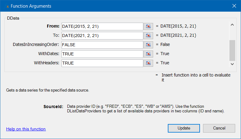
Figure 16: Updating the DData function via the 'Excel Function' dialog box.
Since oil prices are quoted in US dollars, but we are interested in euros, the next step is to determine the historical exchange rates and convert the prices.
To do this, we stay with Federal Reserve Economic Data (FRED), so as to have a single data provider for all time series.
In the table of contents of the Data task pane, we select FRED as the data source and then go to 'Money, Banking & Finance', 'Exchange Rates', and select 'Daily Rates' to have a periodicity consistent with the oil price data. There, we select 'US / EUR Foreign Exchange Rate' by double-clicking the entry.
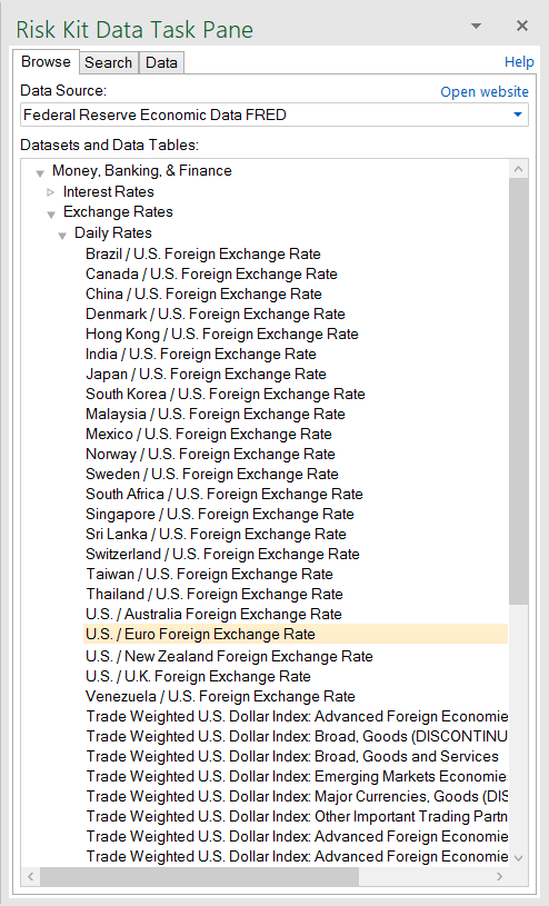
Figure 17: Browsing data tables and sources
To match the time window for the oil prices, we set the filter accordingly and import the data as an array function into our worksheet. Note that the time window specified in one of the previous steps is automatically applied to the newly selected data series.
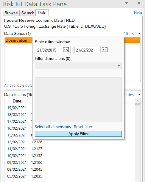
Figure 18: Filtering the target time window
Finally, we select a 1-year EUR interest rate accordingly. In the 'Data' task pane2, we select 'FRED', 'Money, Banking & Finance', 'Interest Rates', 'Interest Rate Swaps' and double-click to select the 1-year tenor on a EUR basis. We filter the target time window as with the previous series and insert the data as an array formula into the worksheet.
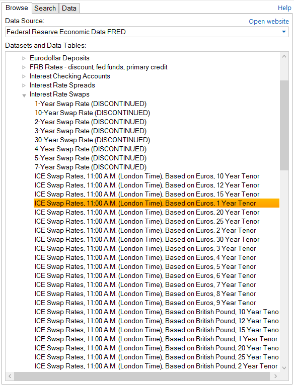
Figure 19: Selecting the swap rates from FRED
Note that the 'From' date and the 'To' date, as the bounds of the time window for the data selection, can be defined by reference. This provides a simple way to build dynamic models that are easy to update. Also, the end date of the series is optional and can therefore be omitted. In this case, the function returns the most recent available data.
In the following example, the reference dates are defined on a central worksheet, 'PARAMS', and then referenced in the formulas.
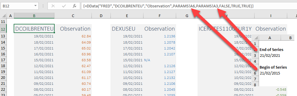
Figure 20: Dynamic linking to data
Synchronizing Time Series
To synchronize the oil prices, exchange rates, and interest rates by date, we use the function 'DDataSync', which returns a union of the date values in the first column and the data series in the subsequent columns. To insert the function, click 'Insert Function' in the ribbon (Figure 1). In the dialog box that opens, select the function 'DDataSync' and click OK.
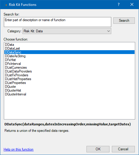
Figure 21: The Risk Kit Data function dialog box.
The function takes the ranges in its first argument. Use the Excel argument separator to delimit the ranges3.
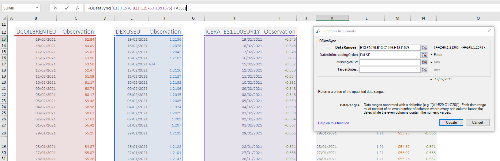
Figure 22: Entering the DDataSync cell function.
By default, the data is sorted in descending order. To invert the order, you can set the 'DatesIncreasingOrder' argument to TRUE (or WAHR in the German version of Excel). In addition, the function interpolates missing values from the nearest neighbors by default. To disable the interpolation, set the 'MissingValue' argument to a non-empty value to be used instead for missing observations. In this particular example, we leave this parameter empty and also keep the descending date order.
Click 'Insert' to insert the function into a cell. Use the function as an array formula, where the number of rows equals the number of data points in the specified data ranges, while the number of columns equals the number of specified data ranges plus one for the date column.
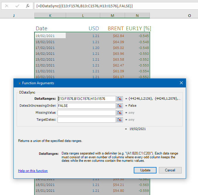
Figure 23: Using the DDataSync cell function.
To further calculate the oil prices in euros, we simply divide the oil price by the exchange rate. We also convert the interest rate from [%] into a plain number by dividing it by 100.
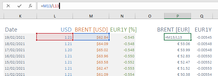
Figure 24: Calculating the oil price in euros.
Calibrating Oil Price and Interest Rate Models
To simulate the oil price and the interest rate as part of the P&L calculation, we need models that allow the price paths to be extrapolated into the future and that fit the historical data and the general properties of the price paths well. We consider a forecast horizon of one year.
Risk Kit offers five process types with calibration, simulation, trends, and confidence bands for the quantiles. These processes have different properties that make them more or less suitable for particular applications.
| Name | Sign | Mean reversion | Long-term growth of percentiles |
| Brownian motion | Both | No | Square root |
| Wiener process | Both | No | Square root plus linear |
| Geometric Brownian motion | Positive | No | Exponential |
| Vasicek process | Both | Yes | Stationary |
| Black-Karasinski process | Positive | Yes | Stationary |
Figure 25: Process types and their properties
For a qualitative choice of process type, it is helpful to plot the process to be calibrated.
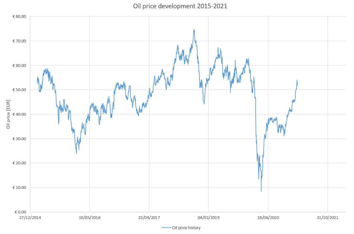
Figure 26: Oil price development
As a commodity price, the oil price typically cannot take on negative values. Therefore, only a geometric Brownian motion or a Black-Karasinski process are suitable.
Within the time window considered, the oil price is also quite stationary, without a clearly recognizable long-term trend.
Once calibrated to the data, both process types produce markedly different forecasts. In particular, the exponentially rising 99% percentiles reach oil price levels that lie far outside the range of the historical data. The confidence bands of the Black-Karasinski process, by contrast, provide moderately conservative coverage of the historical range of the oil price4. We therefore choose the Black-Karasinski model for the 1-year forecast5.
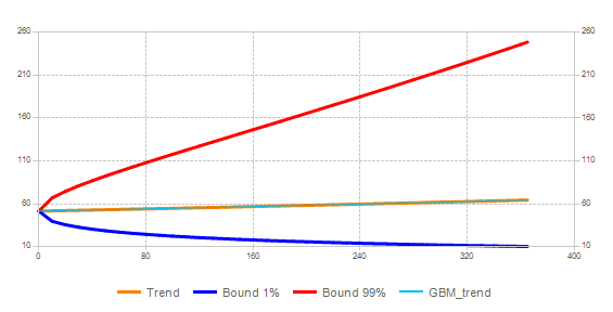
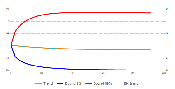
Figure 27: Calibrated geometric Brownian motion and Black-Karasinski process
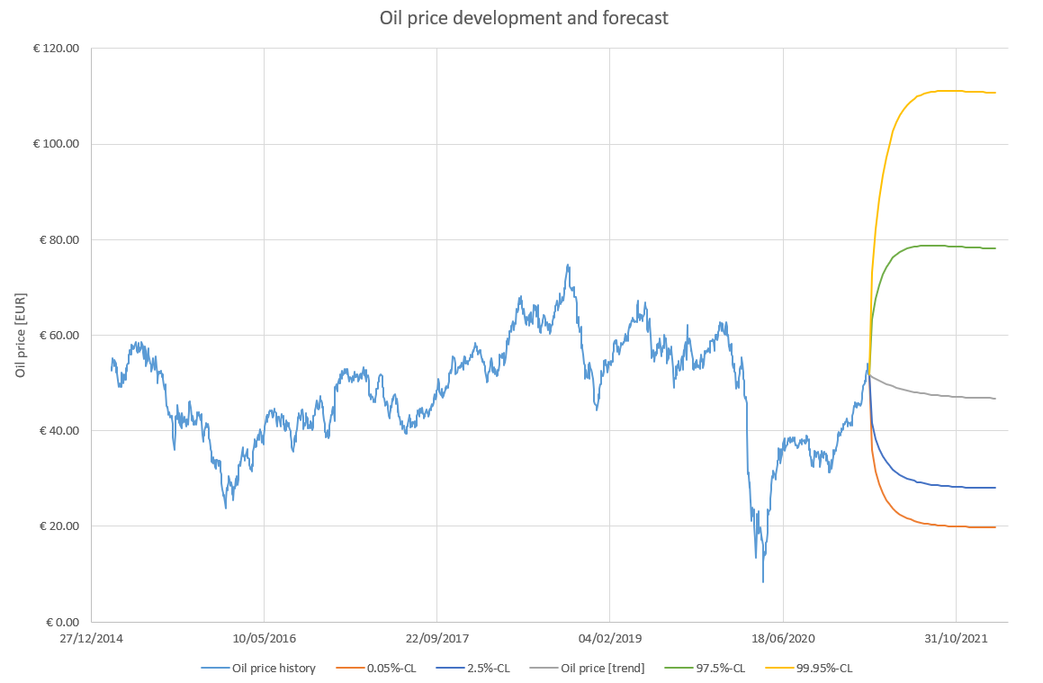
Figure 28: Oil price path and forecast with the Black-Karasinski model
Similarly, we look at the development of interest rates since 2015.
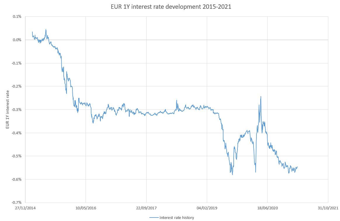
Figure 29: Development of interest rates
Interest rates show quite different properties from commodity prices. In particular, they are currently negative. They also sometimes show episodes of non-stochastic drift, as in the example from 2015, due to central bank interventions. In general, large movements are often accompanied by exogenous shocks.
Since interest rates are a relative quantity, they usually have a stationary long-term trend and do not grow systematically.
Based on these considerations, we choose the Vasicek model for interest rates.
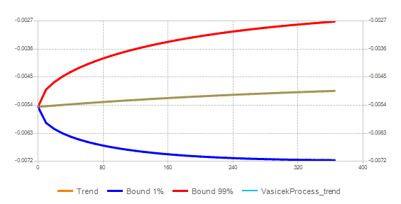
Figure 30: Calibrated Vasicek model for interest rates
Note that the range of the forecast for the next year does not include the interest rate level from early 2015. We accept this model behavior because the movement in 2015 was largely attributable to exogenous factors and central bank policy.
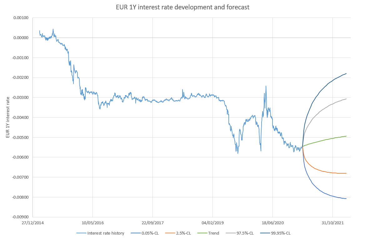
Figure 31: History of interest rates and forecast with the Vasicek model
To calibrate both models for oil prices and interest rates, we use the Risk Kit function 'CalibrateMVProcess'. It estimates the parameters of both processes and the correlations between them, so that the joint behavior of the processes is captured. Note that the function allows each process to have a different type. This makes it possible for oil prices to follow a Black-Karasinski process while interest rates follow a Vasicek process.
The parameter 'DeltaT' assumes that the input time series for the calibration has equidistant time steps. The estimated process parameters are scaled to this time increment.
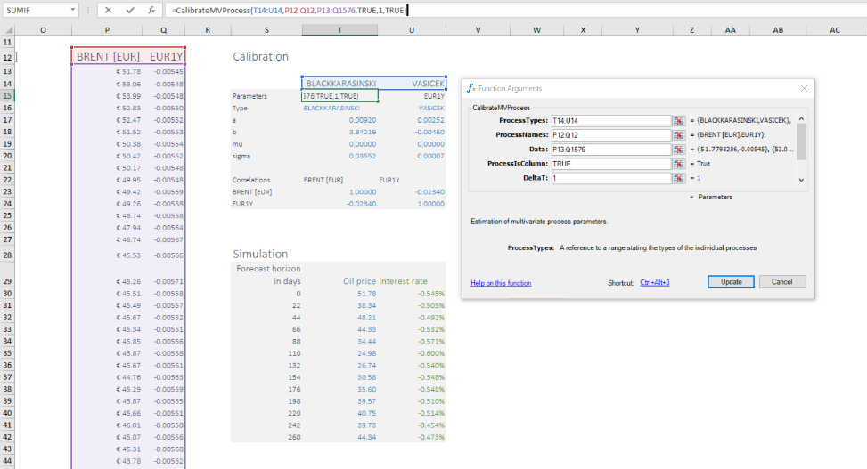
Figure 32: Joint calibration of the two processes
For the simulation, we use the complementary function 'MV_General_path', which uses the parameters in the same order in which the function 'CalibrateMVProcess' returns them.
Note that it is now especially convenient to have the historical price paths in descending date order, since this gives the most recent price, at which the simulation starts, a stable position in the worksheet.
For the simulation, the parameter 'DeltaT' must be chosen the same way as for the calibration in the previous step, since the process parameters are scaled accordingly. The 'times' at which the simulated process is evaluated must be expressed in multiples of 'DeltaT'. So if DeltaT=1 stands for daily data available for 5 business days per week, a one-month forecast has a forecast horizon of 22 business days, and a one-year forecast has one of 260 days.
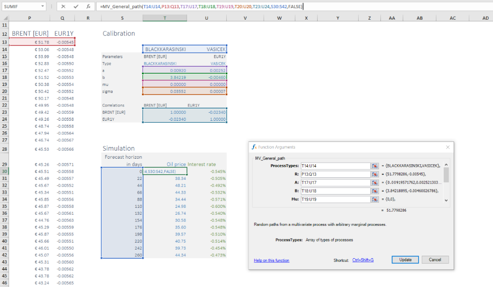
Figure 33: Joint simulation of the two processes
Now we are ready to complete our profit and loss model.
The required amount of oil is uniformly distributed over the interval from 7,500 to 9,500 barrels. We model the random oil price effectively paid over the year as the average oil price over the twelve months.
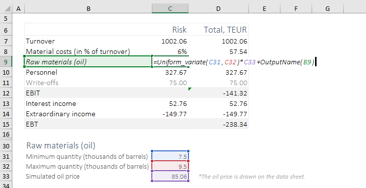
Figure 34: Simulation of raw material costs.
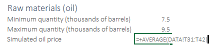
Figure 35: The effectively paid oil price as a 12-month average
We assume that the interest income is determined by the 1Y EUR rate in one year, paid on a notional amount of EUR 10 million.
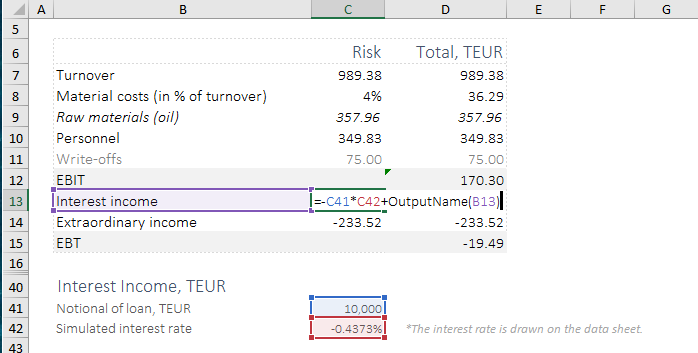
Figure 36: Simulation of interest income
The value of the simulated interest rate is taken from the interest rate path after 260 days.

Figure 37: Referencing the simulated interest rate after 365 days
By analogy, we model the remaining expenses. Personnel costs are specified as a normal distribution with mean 325 and standard deviation 20. In addition, we limit the smallest possible value to 300, meaning that personnel costs below 300 are not simulated.
Extraordinary income arises when one or more counterparties default before paying their invoices. If a default occurs, we assume that the size of the loss is PERT-distributed over a range of 0 to 5, with a most likely value of 3. Since each loss is independent of the others, we use the Compound cell function (Figure 38), which adds up a certain number of random variables. The number of defaults in each fiscal year is Poisson-distributed, with an expected number of 5 defaults.
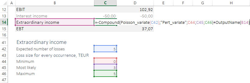
Figure 38: Identifying the extraordinary income.
Monte Carlo Simulation
Before we simulate the model, let us identify the model inputs and outputs. Since we are interested in the behavior of EBIT (D12) and EBT (D15) under the influence of the specified risks, we mark these quantities as model outputs. We are also interested in the effects of the risks on EBIT and EBT. We therefore mark all risks (C7:C10, C13:C14) as inputs.
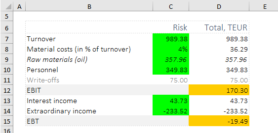
Figure 39: Model inputs and outputs.
To mark the model inputs and outputs, we use the 'Modeling' group in the Risk Kit ribbon.
At this point, the model is fully defined and we can start the simulation. To be able to better interpret the simulation results, however, we carry out a few additional steps6.
First, we attach the function 'Plot' to the output cells to get an impression of the shape of EBIT and EBT. The function takes the output cells as its first argument and displays the results in a window after the simulation.
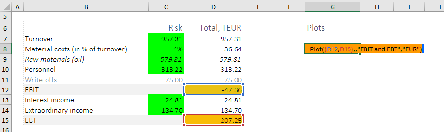
Figure 40: The Plot cell function.
A wide range of optional arguments for the function let you customize the appearance of the charts.
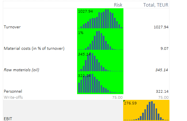
Charts can also be displayed directly in the cell using the function 'PlotInCell' or via the configuration setting 'Show Histograms in Cell'7.
Second, we calculate basic statistics using Risk Kit functions. These functions take the output cell as their first argument and calculate the results after the simulation.
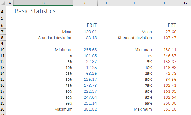
Figure 41: Calculating the statistics.
Third, we specify the cell function 'Sensitivity', which calculates the effects of the model inputs on the respective output.
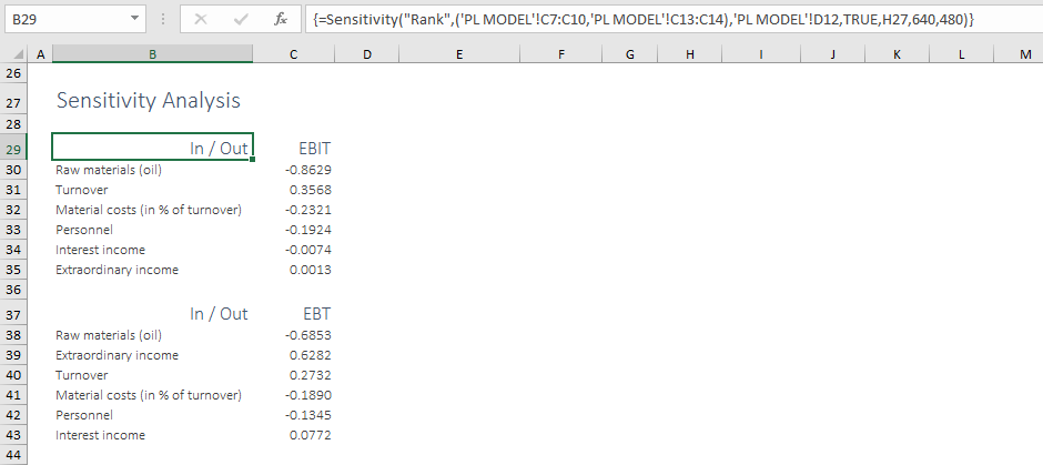
Figure 42: Calculating the sensitivities.
The function 'Sensitivity' can also generate a chart and embed it in the worksheet. To use this feature, set the function's 'CreateChart' argument to TRUE and specify the 'ResultCell' cell in which the chart is embedded, anchored at its top-left corner.
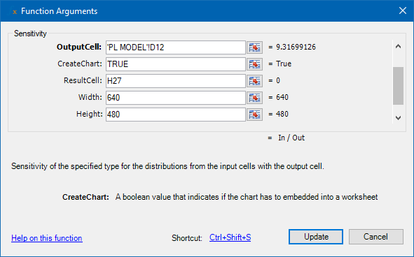
Figure 43: Customizing the 'Sensitivity' function.
Finally, to start the simulation, click 'Simulate' in the Risk Kit ribbon. After the simulation, the add-in displays the EBIT and EBT distributions in a separate window.
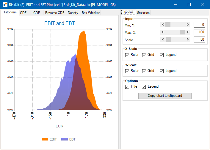
Figure 44: The 'Plot' window.
It also calculates the statistics (Figure 45) and the sensitivities (Figure 47).
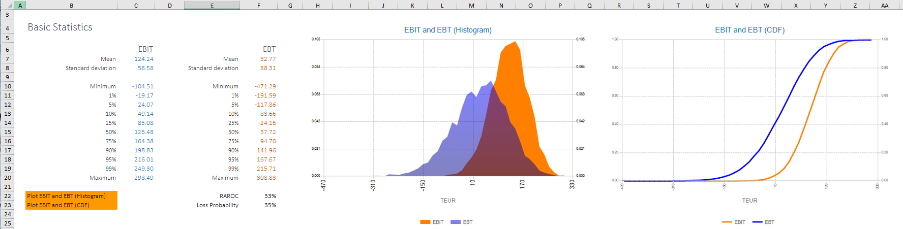
Figure 45: Basic statistics and charts.
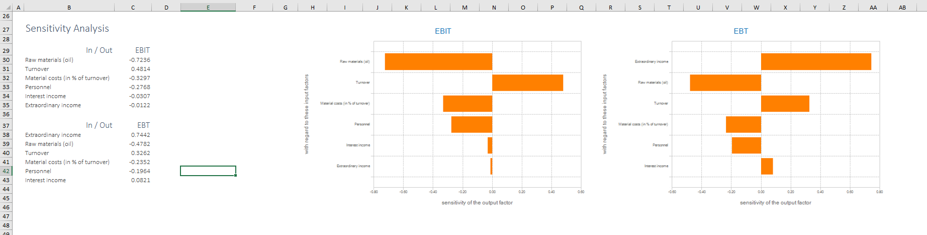
Figure 46: Sensitivity results.
In our example, raw material costs have the largest effect on EBT. In particular, the negative sign of the sensitivity indicates that a rise in the oil price leads to a decline in EBT.
Compared to the raw materials, the effects of the uncertainty in interest rates and interest income are very small.
Conclusion
In this example, we have considered the effects of the oil price in USD on a profit and loss statement in EUR. We have also taken into account the uncertainty in interest rates.
With Risk Kit Data, we were able to find and process historical oil prices, foreign exchange rates, and interest rates quickly and with little effort. The data was synchronized, and missing data was interpolated. Process models were selected and calibrated. Forecasts were simulated and incorporated into the P&L calculation. From the simulation of the P&L model, various statistics, analysis techniques, and charts were derived and presented in a cockpit with interpretable, evaluable results.
This reduces the time and cost involved in sourcing and analyzing data. Through a user-friendly graphical interface, users can browse and aggregate statistics from various sources without needing an extensive technical background.
For questions and comments, please contact us.
1 Note that depending on the language version of Excel you use, booleans may be written differently, for example as WAHR and FALSCH in the German version.
2 See here for details on the ICE rates.
3 The argument separator in Excel depends on the regional settings enabled in the operating system. In German locales, this is usually a semicolon.
4 Note that the sharp drop in oil prices in April 2020, caused by a sudden worldwide lockdown at the start of the COVID-19 pandemic, lies outside the forecast range. We tolerate this deviation of the model, since the price behavior in April/May 2020 is attributable to an exogenous shock, and since, as oil buyers, we are particularly interested in procurement risk.
5 For longer-term forecasts, the strength of the mean reversion, or this property altogether, would have to be reconsidered from scratch.
6 For a detailed discussion and explanation of running a simulation and building a results cockpit, see Wehrspohn/Zhilyakov, Monte Carlo Simulation with Risk Kit, 2021, pp. 26 ff.
7 You will find a detailed description of the in-cell charts in Wehrspohn/Zhilyakov, Monte Carlo Simulation with Risk Kit, 2021, pp. 30 ff. Note that a cell can be marked as both an input and an output cell at the same time, so the distributions in input cells can also be displayed using the 'PlotInCell' function.