
Risk management applications must be able to do justice to both expert assessments of a matter and data analyses, depending on the case at hand.
Standard distributions, however, are usually restricted to a fixed shape with little room for variation. Loosening these restrictions and having more flexible and adaptable tools available has long been a goal for risk managers.
In the Enterprise Risk Evaluator, in Risk Kit, and in our other systems, there is therefore a spectrum of distributions with diverse shapes and properties. The Expert and Poly distributions have now been added. They can be bounded or open at the edges, extend the degrees of freedom available to experts, and adapt to the particularities in the data.
The Expert Distribution
The Expert distribution is a special case of the Poly distributions. It fixes its shape through three quantiles and, if the distribution is meant to be bounded, a minimum and maximum. Conceptually, it is related to the triangular and PERT distributions, but it offers more freedom in shaping its course. For example, it also allows a one-sided or two-sided unbounded representation of impacts. It can therefore be used in areas where a maximum loss cannot easily be specified.
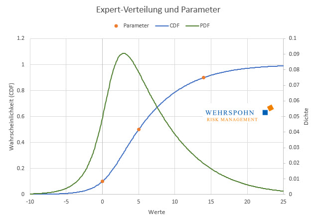
The quantiles used to determine the Expert distribution are symmetric around the median: the p-quantile, the median itself, and the 1-p-quantile. In addition, lower and/or upper bounds for the value range can be specified if needed.
The distribution passes exactly through the specified points.
The Poly Distributions
The Poly distributions are a new[1] and highly flexible tool for describing risks. They derive their adaptability from being built as polynomials. Similar to how a Taylor series of sufficiently high degree can approximate continuous and smooth functions to any desired accuracy, Poly distributions adapt to data or expert assessments in great detail.[2]
Poly distributions can take on any shape at their boundaries. They can be unbounded on both sides (Poly), bounded on the left or right (PolyL and PolyR respectively), or bounded on both sides (PolyLR).
The coefficients of the polynomials are abstract and not accessible to experts. When the distributions are parameterized using expert assessments, this is therefore done through a list of quantiles, that is, pairs of values and probabilities, in the function CalibratePoly, which determines the polynomial coefficients from the quantiles.
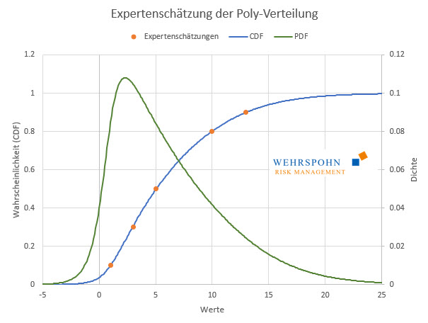
Unlike the Expert distribution, a special case of the Poly distribution, the quantiles do not need to be symmetric around the median but can be chosen freely. The list must contain at least three points and can contain any number of points beyond that. In addition, lower and upper bounds can be specified if needed. The distribution is chosen so that it fits the specified points as seamlessly as possible. Bounds are always matched exactly.[3]
The second important application of Poly distributions is fitting them to data. For observed data, this goes without saying. But simulated data also play an important role.
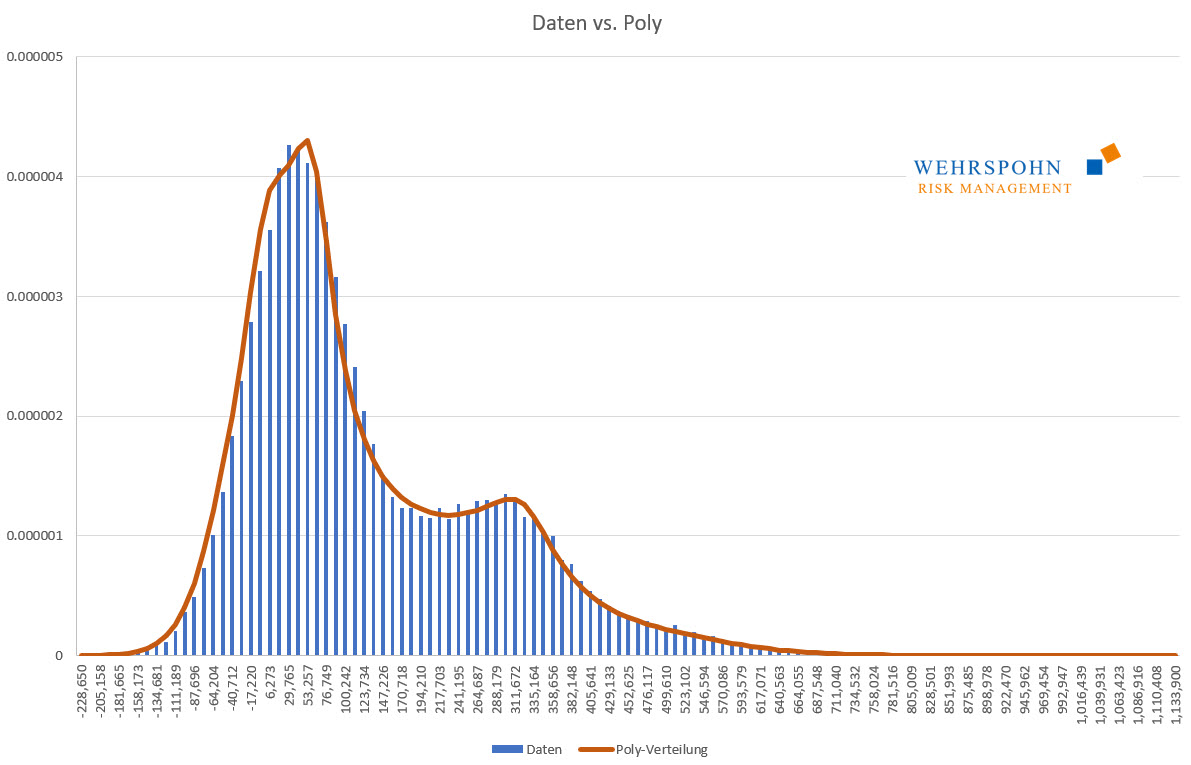
In ERM, all material risks of a company are meant to be considered together in a single analysis. However, many companies have specific risk types that are important enough to receive separate attention, with dedicated systems used for this risk type that run their own simulations. Typical examples are treasury applications or commodity procurement.
With Poly distributions, the results of specialized simulations can be transferred into ERM very precisely and with very little effort. This is true even when the simulated distributions have a shape that cannot be represented with a standard distribution, for example when they have multiple modes. In simulated distributions, multiple modes arise naturally when major risks or crises occur in the simulation.
Poly distributions are a universal key. Thanks to their flexibility, given a sufficiently high degree n of the polynomial, they can bring out particularities in the data that other distributions cut off.
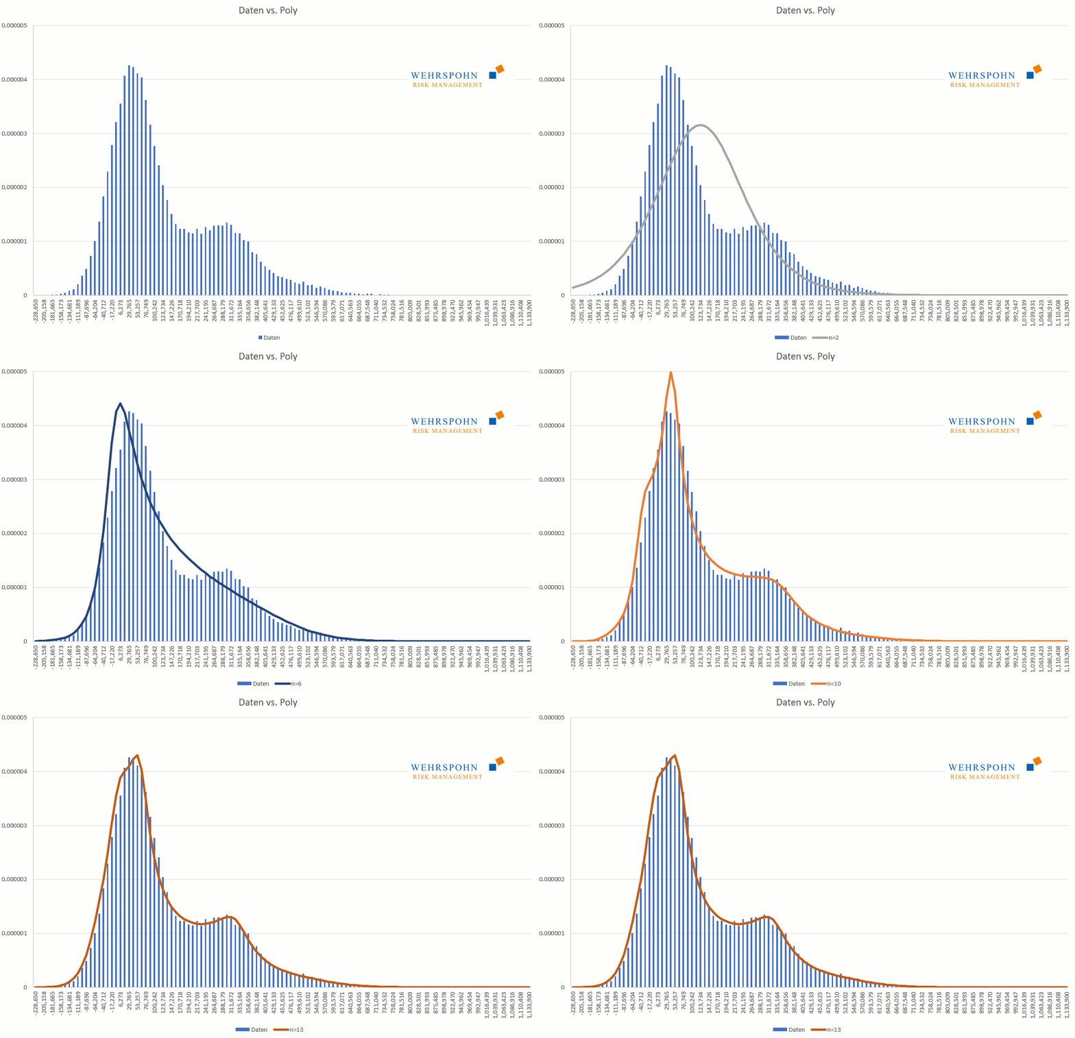
They can also fit many standard distributions so closely that, for practical purposes, they can no longer be distinguished from them.
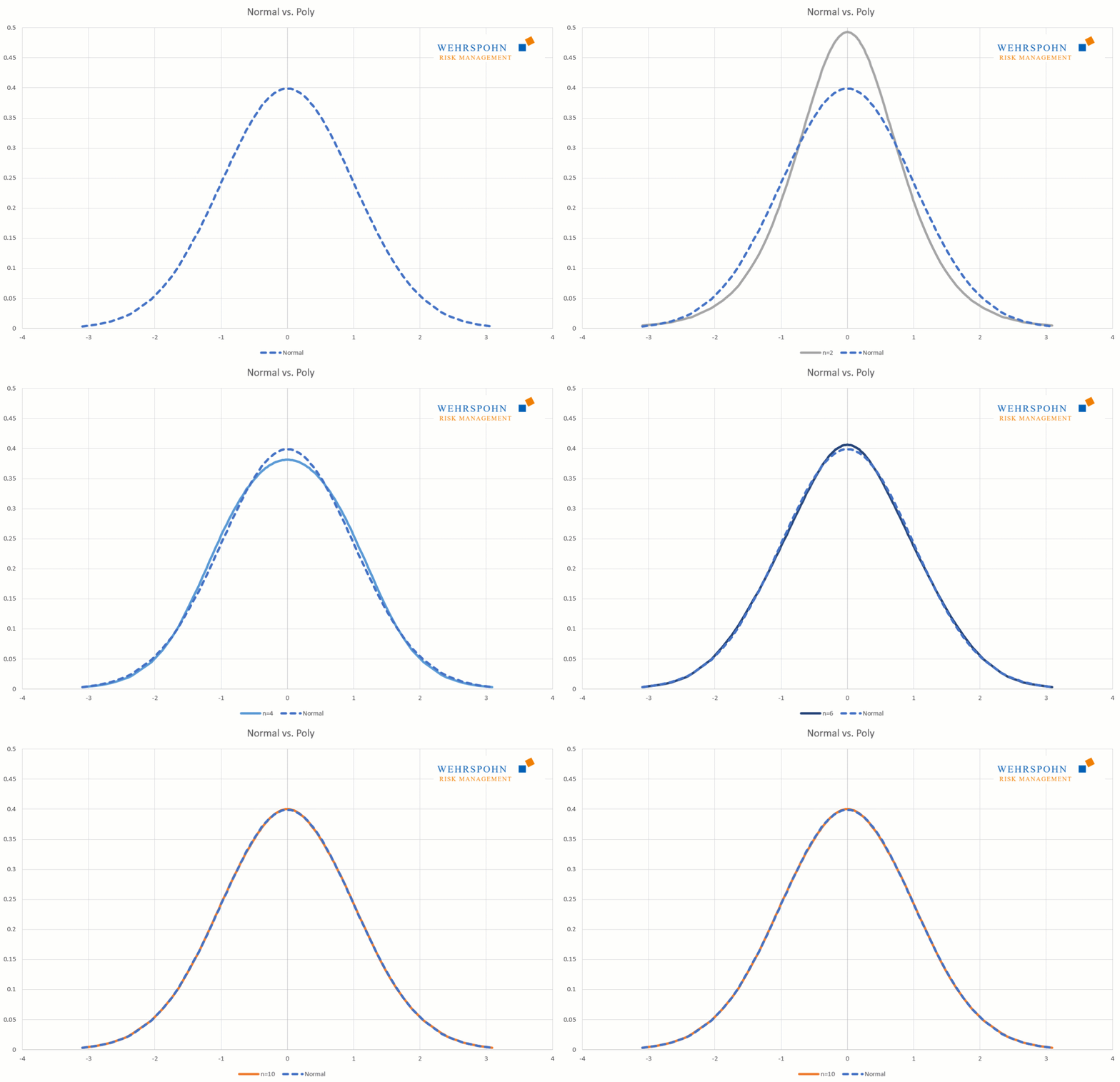
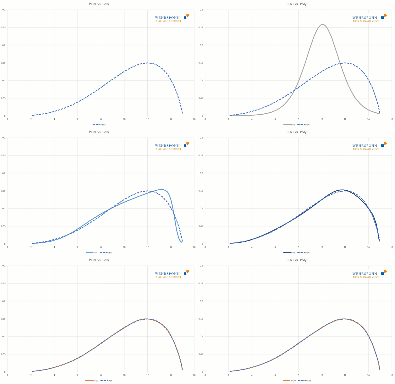
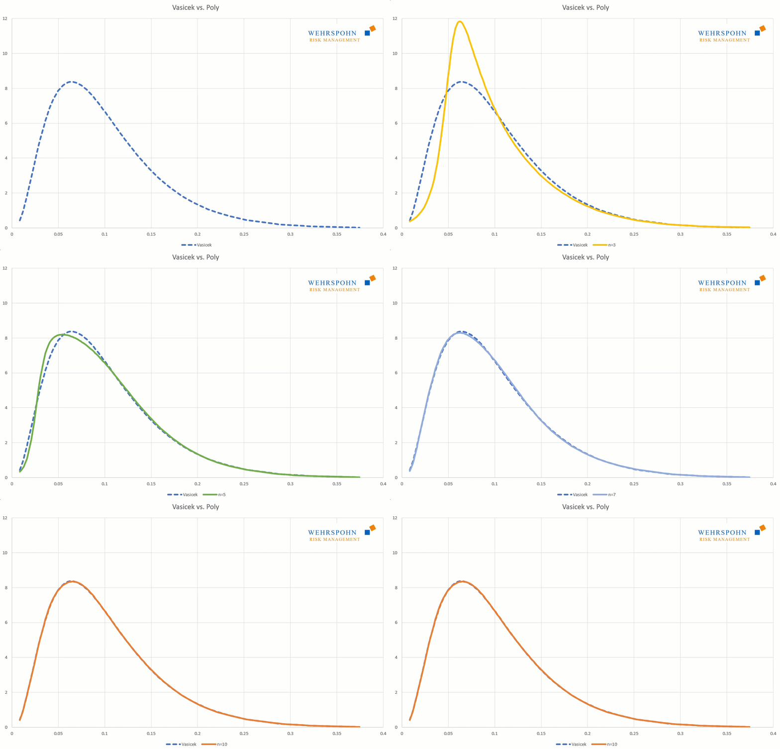
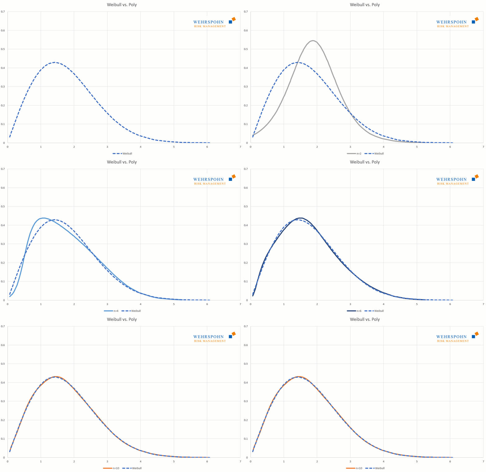
[1] They were introduced by Thomas Keelin under the name Metalog distributions. See Thomas W. Keelin (2016) The Metalog Distributions. Decision Analysis 13(4):243-277.
[2] The only requirement is that the underlying relationship is continuous and has finite moments. That is, the expected value, variance, and so on should exist, and there should be no jumps or spikes.
[3] The maximum order can be controlled to avoid potential overfitting.